Week 7 - Simulation of a 1D Super-sonic nozzle flow simulation using Macormack Method

Aim: To Simulate the isentropic flow through a Quasi 1D subsonic nozzle by deriving both the conservation and non-conservation forms of the governing equations and solve them by implementing MacCormack's technique using MATLAB.

Mac-Cormack‟s technique is a variation of the LaxWendroff Approach in which the latter‟s complex second-order derivative is replaced by forwarding differences on the predictor and rearward differences on the corrector. Mac-Cormack‟s scheme is perfectly satisfactory and the results have been known to be approximately correct for many fluid flow applications.

Governing Equations:

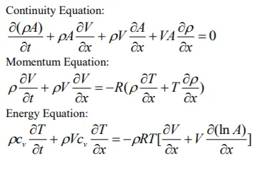
The fluid flow through the nozzle is governed by continuity, momentum, and energy equations. Since the flow is assumed to
be quasi-One dimensional flows, the conventional equations are slightly modified, and Non-Conservation equations as suitable to unsteady, quasi-one-dimensional flow:

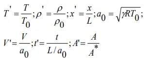
The following non-dimensional parameters:

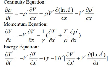
The governing equations are modified using Non-Dimensional Numbers:

Macroman Scheme:

It‟s a two-step Predictor-Corrector formula. The Predictor formula has been implemented using forward
difference. The corrector formula is implemented using the rearward difference method.

Main code

clear all
close all
clc

n=31; %bo:of grid points
gamma=1.4;
x=linspace(0,3,n);
dx=x(2)-x(1);

nt=1400; %time step
C=0.5;   %courant number

%function non conservatve
tic;
[Mass_flow_rate_NC,Pressure_NC,Mach_number_NC,rho_NC,v_NC,T_NC,rho_throat_NC,v_throat_NC,T_throat_NC,Mass_flow_rate_throat_NC,Pressure_throat_NC,Mach_number_throat_NC]=Non_conservative_form(x,dx,n,gamma,nt,C);
Time_elapsed_NC=toc;
fprintf('time elapsed non conservative',Time_elapsed_NC);
hold on

%plotting
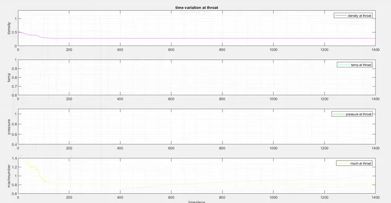
figure(2)

%density
subplot(4,1,1)
plot(linspace(1,nt,nt),rho_throat_NC,'color','m')
ylabel('density')
legend({'density at throat'});
axis([0 1400 0 1.3]);
grid minor;
title('time variation at throat')

%temperature
subplot(4,1,2)
plot(linspace(1,nt,nt),T_throat_NC,'color','c')
ylabel('temp')
legend({'temp at throat'});
axis([0 1400 0.6 1]);
grid minor;

%pressure
subplot(4,1,3)
plot(linspace(1,nt,nt),Pressure_throat_NC,'color','g')
ylabel('pressure')
legend({'pressure at throat'});
axis([0 1400 0.4 1.1]);
grid minor;

%machnumber
subplot(4,1,4)
plot(linspace(1,nt,nt),Mach_number_throat_NC,'color','y')
xlabel('timesteps')
ylabel('machnumber')
legend({'mach at throat'});
axis([0 1400 0.6 1.4]);
grid minor;

%primitive values for nc
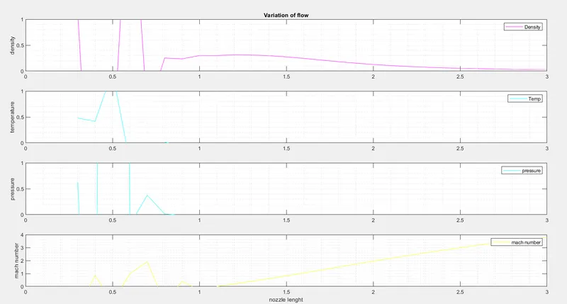
figure(3);

%density
subplot(4,1,1);
plot(x,rho_NC,'color','m')
ylabel('density')
legend({'Density '});
axis([0 3 0 1]);
grid minor;
title('Variation of flow')

%temperature
subplot(4,1,2)
plot(x,T_NC,'color','c')
ylabel('temperature')
legend({'Temp'});
axis([0 3 0 1])
grid minor;

%pressure
subplot(4,1,3)
plot(x,Pressure_NC,'color','c')
ylabel('pressure')
legend({'pressure'});
axis([0 3 0 1])
grid minor;

%mach number
subplot(4,1,4)
plot(x,Mach_number_NC,'color','y')
xlabel('nozzle lenght')
ylabel('mach number')
legend({'mach number'});
axis([0 3 0 4])
grid minor;


%function conservative
tic;
[Mass_flow_rate_C,Pressure_C,Mach_number_C,rho_C,v_C,T_C,rho_throat_C,v_throat_C,T_throat_C,Mass_flow_rate_throat_C,Pressure_throat_C,Mach_number_throat_C]=Conservative_form(x,dx,n,gamma,nt,C);
Time_elasped_C=toc;
fprintf('Time elapsed conservative',Time_elapsed_C)

%plotting
figure(5)
%density
subplot(4,1,1)
plot(rho_throat_C,'color','m')
ylabel('density')
legend({'Density at throat'});
axis([0 1400 0 1]);
grid minor;
title('Timestep-Conservative')

%temperature
subplot(4,1,2)
plot(T_throat_C,'color','c')
ylabel('temperature')
legend({'Temp at throat'});
axis([0 1400 0.6 1]);
grid minor;

%pressure
subplot(4,1,3)
plot(Pressure_throat_C,'color','g')
ylabel('pressure')
legend({'pressure at throat'});
axis([0 1400 0.2 0.8]);
grid minor

%mach number
subplot(4,1,3)
plot(Mach_number_throat_C,'color','y')
xlabel('timesteps')
ylabel('mach number')
legend({'mach at throat'});
axis([0 1400 0.6 1.4]);
grid minor;

%simulation for primarary value for nc form
figure(6);

%density
subplot(4,1,1)
plot(x,rho_C,'color','m')
ylabel('density')
legend({'Density '});
axis([0 3 0 1]);
grid minor;
title('Variation of flow')

%temperature
subplot(4,1,2)
plot(x,T_C,'color','c')
ylabel('temperature')
legend({'Temp'});
axis([0 3 0 1])
grid minor;

%pressure
subplot(4,1,3)
plot(x,Pressure_C,'color','c')
ylabel('pressure')
legend({'pressure'});
axis([0 3 0 1])
grid minor;

%mach number
subplot(4,1,4)
plot(x,Mach_number_C,'color','y')
xlabel('nozzle lenght')
ylabel('mach number')
legend({'mach number'});
axis([0 3 0 4])
grid minor;

%comparison
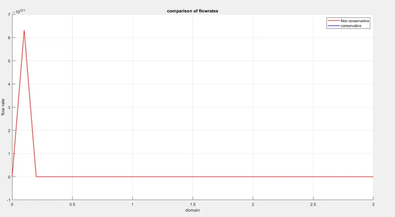
figure(7)
hold on
plot(x,Mass_flow_rate_NC,'r','linewidth',1.25)
hold on;
plot(x,Mass_flow_rate_C,'b','linewidth',1.25)
hold on;
grid on

legend('Non conservative','conservative');
xlabel('domain')
ylabel('flow rate')
title('comparison of flowrates');

Non conservative function

%function for nc form

function[Mass_flow_rate_NC,Pressure_NC,Mach_number_NC,rho_NC,v_NC,T_NC,rho_throat_NC,v_throat_NC,T_throat_NC,Mass_flow_rate_throat_NC,Pressure_throat_NC,Mach_number_throat_NC]=Non_conservative_form(x,dx,n,gamma,nt,C)

%intials

rho_NC=1-0.3146*x;
T_NC=1-0.2341-x;
v_NC=(0.1+1.09*x).*T_NC.^0.5;

%area throat profiles
a=1+2.2*(x-1.5).^2;
throat=find(a==1);

%outer time
for k=1:nt
    dt=min(C.*dx./(sqrt(T_NC)+v_NC));
    %creating temp value fpr storing
    rho_old=rho_NC;
    T_old=T_NC;
    v_old=v_NC;
    
    %predictor
    for j=2:n-1
        dv_dx=(v_NC(j+1)-v_NC(j))/dx;
        drho_dx=(rho_NC(j+1)-rho_NC(j))/dx;
        dT_dx=(T_NC(j+1)-T_NC(j))/dx;
        dlog_a_dx=(log(a(j+1))-log(a(j)))/dx;
        
        %continuity
        drho_dt_P(j)= -rho_NC(j)*dv_dx-rho_NC(j)*v_NC(j)*dlog_a_dx-v_NC(j)*drho_dx;
        %momentum
        dv_dt_P(j)= -v_NC(j)*dv_dx - (1/gamma)*(dT_dx+(T_NC(j)*drho_dx/rho_NC(j)));
        %energy
        dT_dt_P(j)= -v_NC(j)*dT_dx -(gamma-1)*T_NC(j)*(dv_dx+v_NC(j)*dlog_a_dx);
        
        %solution 
        rho_NC (j) = rho_NC(j) + drho_dt_P(j)*dt;
        v_NC(j)= v_NC(j) + dv_dt_P(j)*dt;
        T_NC(j)= T_NC (j) + dT_dt_P(j)*dt;
        
    end
    %corrector method
    for j=2:n-1
    dv_dx = (v_NC(j) - v_NC(j-1))/dx;
    drho_dx = (rho_NC(j) - rho_NC(j-1))/dx;
    dT_dx = (T_NC(j) - T_NC(j-1))/dx; 
    dlog_a_dx = (log(a(j))-log(a(j-1)))/dx;
    
    %contunity
    drho_dt_C(j) = -rho_NC(j)*dv_dx - rho_NC(j)*v_NC(j)*dlog_a_dx - v_NC(j)*drho_dx;
    %momentum
    dv_dt_C(j) = -v_NC(j)*dv_dx - (1/gamma)*(dT_dx + (T_NC(j)*drho_dx/rho_NC(j)));
    %energy
    dT_dt_C(j) = -v_NC(j)*dT_dx - (gamma - 1) *T_NC(j)*(dv_dx + v_NC(j) *dlog_a_dx);
    
    end
    drho_dt=0.5.*(drho_dt_P + drho_dt_C);
    dv_dt= 0.5.*(dv_dt_P + dv_dt_C);
    dT_dt=0.5.*(dT_dt_P + dT_dt_C);
    
    %final
    for i=2:n-1
        rho_NC(i) = rho_old(i) + drho_dt(i)*dt;
        v_NC(i) = v_old(i) + dv_dt(i)*dt;
        T_NC(i) =T_old(i) + dT_dt(i)*dt;
        
    end
    %inlet
    rho_NC(1)=1;
    v_NC(1)= 2*v_NC(2) - v_NC(3);
    T_NC(1) = 1;
    %outlet
    rho_NC(n)=2*rho_NC(n-1)- rho_NC(n - 2); 
    v_NC(n)= 2*v_NC(n-1) - v_NC(n-2);
    T_NC(n)= 2*T_NC(n - 1)- T_NC(n - 2);
    
    Mass_flow_rate_NC= rho_NC.*a.*v_NC;
    Pressure_NC=rho_NC.*T_NC;
    Mach_number_NC=(v_NC./sqrt (T_NC));
    
    %calculating variable
    rho_throat_NC(k)=rho_NC(throat);
    T_throat_NC(k)= T_NC(throat);
    v_throat_NC(k) =v_NC(throat);
    Mass_flow_rate_throat_NC(k)= Mass_flow_rate_NC(throat);
    Pressure_throat_NC(k)= Pressure_NC(throat);
    Mach_number_throat_NC(k)= Mach_number_NC(throat);
    
    %plotting
    figure(1);
    if k==50
        plot(x,Mass_flow_rate_NC,'m','linewidth',1.25);
        hold on
    elseif k==100
         plot(x,Mass_flow_rate_NC,'c','linewidth',1.25);
         hold on
    elseif k==200
         plot(x,Mass_flow_rate_NC,'g','linewidth',1.25);
         hold on
    elseif k==400
         plot(x,Mass_flow_rate_NC,'y','linewidth',1.25);
         hold on
    elseif k==800
         plot(x,Mass_flow_rate_NC,'k','linewidth',1.25);
         hold on
    end
    
    %label
    title('mass flow -NC')
    xlabel('distance')
    ylabel('mass flow rate')
    legend({'timesteps'})
    axis([0 3 0 2])
    grid on
    
end
end

conservative

%conservative form

function[Mass_flow_rate_C,Pressure_C,Mach_number_C,rho_C,v_C,T_C,rho_throat_C,v_throat_C,T_throat_C,Mass_flow_rate_throat_C,Pressure_throat_C,Mach_number_throat_C]=Conservative_form(x,dx,n,gamma,nt,C)

for i=1:n
    if (x(i) >=0 && x(i)<=0.5)
        rho_C(i)=1;
        T_C(i)=1;
    elseif (x(i) >=0.5&&x(i)<=1.5)
        rho_C(i)=1-0366*(x(i)-0.5);
        T_C(i)=1-0.167*(x(i)-0.5);
    elseif(x(i) >=1.5 && x(i)<=3)
        rho_C(i)=0.634-0.3879*(x(i)-1.5);
        T_C(i)=0.833-0.3507*(x(i)-1.5);
    end
end
%area
a=1+2.2*(x-1.5).^2;
throat=find(a==1);

%intial
v_C=0.59./(rho_C.*a);
Pressure_C=rho_C.*T_C;

%intial vector
U1 = rho_C.*a;
U2 = rho_C.*a.*v_C;
U3 = rho_C.*a.* (T_C./(gamma-1)) + ((gamma/2).*v_C.^2);

%outer time loop
for k= 1:nt
    dt=min(C.*dx./(sqrt(T_C)+v_C));
    U1_old=U1;
    U2_old=U2;
    U3_old=U3;
    %calculating flux vector
    F1=U2;
    F2 = ((U2.^2)./U1) + ((gamma-1)/gamma)*(U3- (gamma/2)*((U2.^2)./U1));
    F3 = ((gamma*U2.*U3)./U1) (gamma*(gamma-1)*((U2.^3)./(2*U1.^2)));
    
    %predictor
    for j=2:n-1
        J2(j) = (1/gamma)*rho_C(j)*T_C(j)*((a(j + 1) - a(j))/dx);
        %continuity
        dU1_dt_P(j) = -((F1(j+1) - F1(j))/dx);
        %momentum
        dU2_dt_P(j)= -((F2(j+1)-F2(j))/dx) + J2(j);
        %energy
        dU3_dt_P(j)= -((F3(J+1)-F3(j))/dx);
        
        U1(j)=U1(j)+dU1_dt_P(j)*dt;
        U2(j)=U2(j)+dU2_dt_P(j)*dt;
        U3(j)=U3(j)+dU3_dt_P(j)*dt;
    end
    F1=U2;
    F2=((U2.^2)./U1) + ((gamma-1)/gamma)*(U3 -((gamma*0.5*(U2.^2))./(U1)));
    F3 = ((gamma*U2.*U3)./U1)-((gamma*0.5*(gamma-1)*(U2.^3))./(U1.^2));
    
    %CORRECTOR
    for j=2:n-1
        J2(j)=(1/gamma)*rho_C(j)*T_C(j)*((a(j)-a(j-1))/dx);
        
        dU1_dt_C(j)=-((F1(j)-F1(j-1))/dx);
        dU2_dt_C(j)=-((F2(j)-F2(j-1))/dx)+J2(j);
        dU3_dt_C(j)=-((F3(j)-F3(j-1))/dx);
        
    end
    %time derivative
    dU1_dt=0.5*(dU1_dt_P+dU1_dt_C);
    dU2_dt=0.5*(dU2_dt_P+dU2_dt_C);
    dU3_dt=0.5*(dU3_dt_P+dU3_dt_C);
    
    %final soln
    for i=2:n-1
        U1(i)=U1_old(i)+dU1_dt(i)*dt;
        U2(i)=U2_old(i)+dU2_dt(i)*dt;
        U3(i)=U3_old(i)+dU3_dt(i)*dt;
    end
    %inlet
    U1(1)=rho_C(1)*a(1);
    U2(1)=2*U2(2)-U2(3);
    v_C(1)=U2(1)./U1(1);
    U3(1)=U1(1)*((T_C(1)/(gamma-1))+((gamma/2)*(v_C(1)).^2));
    %outlet
    U1(n)=2*U1(n-1)-U1(n-2);
    U2(n)=2*U2(n-1)-U2(n-2);
    U3(n)=2*U3(n-1)-U3(n-2);
    
    %final value 
    rho_C=U1./a;
    v_C=U2./U1;
    T_C=(gamma-1)*((U3./U1-(gamma/2)*(v_C).^2));
    
    %defining
    Mass_flow_rate_C=rho_C.*a.*v_C;
    Pressure_C=rho_C.*T_C;
    Mach_number_C=(v_C./sqrt(T_C));
    
    %calculating
    rho_throat_C(k)=rho_C(throat);
    T_throat_C(k)= T_C(throat);
    v_throat_C(k) =v_C(throat);
    Mass_flow_rate_throat_C(k)= Mass_flow_rate_C(throat);
    Pressure_throat_C(k)= Pressure_C(throat);
    Mach_number_throat_C(k)= Mach_number_C(throat);
    
    %plotting
    figure(4)
    if k==50
        plot(x,Mass_flow_rate_C,'m','linewidth',1.25);
        hold on
    elseif k==100
         plot(x,Mass_flow_rate_C,'c','linewidth',1.25);
         hold on
    elseif k==200
         plot(x,Mass_flow_rate_C,'g','linewidth',1.25);
         hold on
    elseif k==400
         plot(x,Mass_flow_rate_C,'y','linewidth',1.25);
         hold on
    elseif k==800
         plot(x,Mass_flow_rate_C,'k','linewidth',1.25);
         hold on
    end
    
    %label
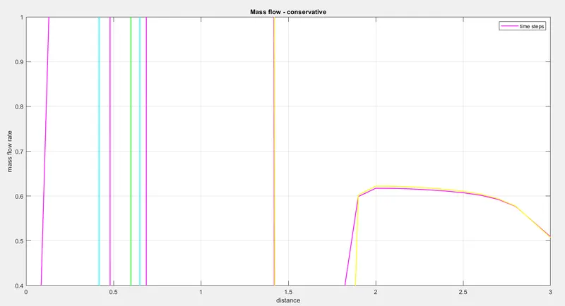
    title('Mass flow - conservative')
    xlabel('distance')
    ylabel('mass flow rate')
    legend('time steps')
    axis([0 3 0.4 1])
    grid on
end
end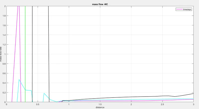

RESULT: conservative form faster than non-conservative form