FVM Literature Review

Finite Volume Method:

The Finite Volume Method (FVM) is a numerical technique that transforms the partial differential equations representing conservative laws over differential volume into discrete algebraic equations over finite volumes (elements or cells).

It is similar to the finite element method.

Whereas in FVM, the solution is discretized into non-overlapping elements or finite volumes. The partial differential equations are then discretized/transformed into algebraic equations by integrating them over each discrete element. The system of algebraic equations is then solved to compute the values of the dependent variable for each of the elements.

In FVM, some of the terms in the conservation equation are turned into face fluxes and evaluated at the finite volume faces. Because the flux
entering a given volume is identical to that leaving the adjacent volume.

Advantages:

• Fluxes are identical in a given volume at entry and outlet.
• FVM is strictly conservative.
• The inherent conservative property of FVM makes it a preferred method.
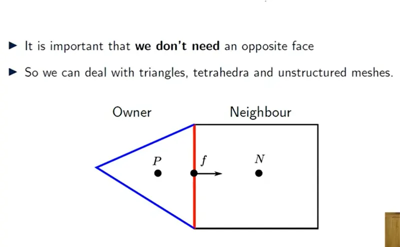
• It can be formulated in the physical space on unstructured polygonal meshes.
• Easy to implement a variety of boundary conditions in a non-invasive manner, since the unknown variables are evaluated at the centroids of the volume elements, not at their boundary faces.
• It is quite suitable for the numerical simulation of a variety of applications involving fluid flow and heat and mass transfer, and developments in the method have been closely entwined with advances in CFD.

The Finite Difference Method Vs Finite Volume Method:

FDM discretization is based upon the differential form of the PDE to be solved. Each derivative is replaced with an approximate difference formula (that can generally be derived from a Taylor series expansion). The computational domain is usually divided into cells (the grid), and the solution will be obtained at each nodal point. The FDM is easiest to understand when the physical grid is Cartesian, but through the use of curvilinear transforms the method can be extended to domains that are not easily represented by brick-shaped elements. The discretization results in a system of equations of the variable at nodal points, and once a solution is found, then we have a discrete representation of the solution.

FVM discretization is based upon an integral form of the PDE to be solved (e.g. conservation of mass, momentum, or energy). The PDE is written in a form that can be solved for a given finite volume (or cell). The computational domain is discretized into finite volumes and then for every volume, the governing equations are solved. The resulting system of equations usually involves fluxes of the conserved variable, and thus the calculation of fluxes is very important in FVM.

The basic advantage of this method over FDM is it does not require the use of structured grids, and the effort to convert the given mesh into a structured numerical grid internally is completely avoided. As with FDM, the resulting approximate solution is discrete, but the variables are typically placed at cell centers rather than at nodal points. This is not always true, as there are also face-centered finite volume methods. In any case, the values of field variables at non-storage locations (e.g. vertices) are obtained using interpolation.

Needs of Interpolation schemes:

Interpolation schemes:

In order to interpolate data from the coarse grid to the fine one in the best possible way, a "conservative" interpolation formula has been developed.

Different CFD codes offer different types of discretization schemes.

Finite Volume uses an integral form of the conservation equation.

Types of interpolation schemes:

• Upwind interpolation.
• Central Differencing Schemes or Linear interpolation.
• Linear upwind interpolation.
• QUICK
• Limited linear.

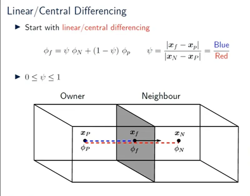
Central Differencing Schemes or Linear interpolation:

• Approximate the value of the variable at the CV face center by linear interpolation values at two nearest nodes.
• This scheme is second-order accurate.
• Variation between centroid is linear

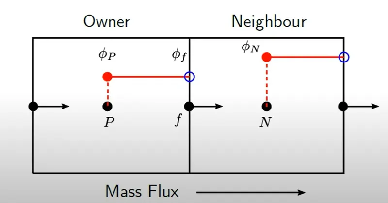
Upwind Interpolation:

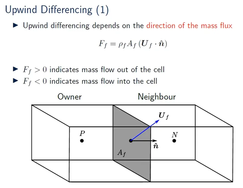
• Mass flux no longer varies linearly across the cell face.
• Mass flux is constant between the cell face and cell centroid.
• upwind is only first order accuracy.
• It is stable for only convection dominant flow.

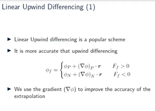
Linear upwind interpolation:

• It is second-order accurate.
• It is popular for convection terms.

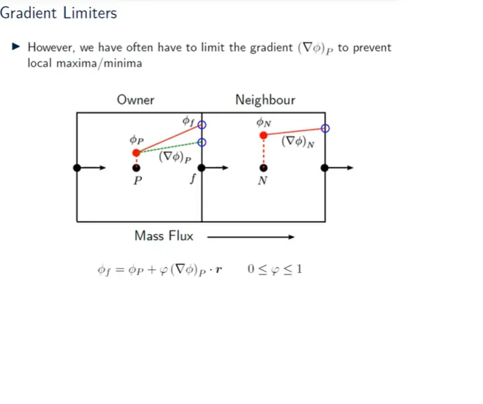
Flux Limiters

Numerical flux function of the high-resolution conservative scheme as

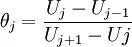
where are the numerical flux of conservative low order and high order schemes respectively and is a function of smoothness parameter usually defined as

Defining the limiter function in such a way that it satisfies at least the following properties:

• remains positive,
• satisfies
• passes through a particular region known as the TVD region associated with the underlying scheme in order to guarantee the stability of the scheme.