Solving the steady and unsteady 2D heat conduction problem
Aim:
To solve 2D steady-state and Unsteady state heat conduction by using iterative solvers like Jacobi, gauss seidel, and Successive overrelaxation methods.
Given:
- Top boundary - 600k
- Bottom boundary - 900k
- Left boundary - 400k
- Right boundary - 800k
- Absolute error - 1e-4.
Assumption:
- The computation area is considered to be a square.
- Row and columns are equal because it is square(nx=ny).
- Temperatures at the corners are the summation of the nearest temperatures.
- error=9e9.
- timestep=dt=1e-3.
- alpha=1.4= diffusion coefficient
- omega=1.5 Rexalation coefficient
Theory:
2 D Steady and Unsteady state heat conduction without considering Internal energy:
Unsteady state heat conduction :
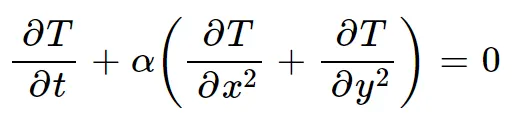
for steady-state heat conduction,
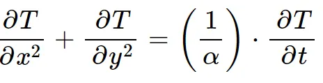 ,
,
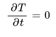 ,
,
therefore Steady-state heat conduction,
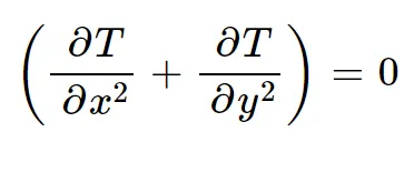
Boundary Nodes:
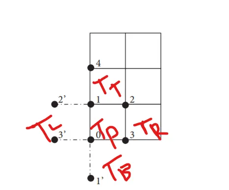
Solving steady-state heat conduction equation:
Discretization of Steady-state heat conduction equation without an internal heat source in geometry and Time domain. Step length of the domain is uniform discretized ie dx=x2-x1, dy=y2-y1
the steady-state equation is discretized using a Central differencing scheme,
Jacobi Method:
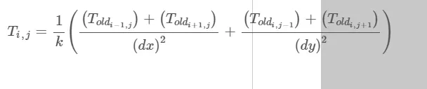
Gauss-Seidel Method:

This method uses values from previous iterations.
SOR:(Successive Over-relaxation)
In this method a scaling factor is used to make the process faster than Jacobi and Gauss_seidel, Hence it has fewer number iteration.

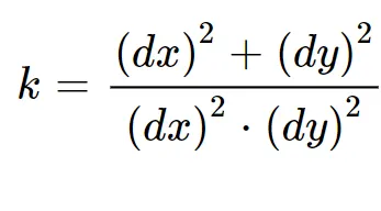
In above all method the value of K is
Solving unsteady or Transient heat conduction equation:(Explicit)
Discretization of unsteady-state heat conduction equation without an internal heat source in geometry and Time domain. Step length of the domain is uniform discretized ie dx=x2-x1, dy=y2-y1
the unsteady-state equation is discretized using a Central differencing scheme,

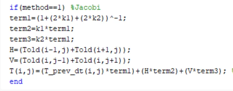
Solving Unsteady state heat conduction:(Implicit)
Program:
%Steady state heat conduction

clear all
close all
clc

%Inputs
nx = 10;
ny = nx;
T = ones(nx,ny);
l=1;
x=linspace(0,l,nx);
y=linspace(0,l,ny);
dx=l/(nx-1);
dy=l/(ny-1);
%Boundary conditions
TL = 400;
TR = 800;
TT = 600;
TB = 900;

%Creating Domain
T(:,1) = TL;
T(:,end)= TR;
T(1,:)=TT;
T(end,:)=TB;

%Summation of Temperatures at corner
T(1,1)=500;
T(1,10)=700;
T(10,1)=650;
T(10,10)=850;

%Initial value of T
T_initial = T;
T_old=T;

% Assigning error and Tolerance
tolerance=1e-4;
error=9e9;
dt=1e-3;% timestep
alpha=1.4;% diffusion coefficient
omega=1.5;


 % calculating 2D steady state heat conduction by Jacobi method

jacobian_iteration=1;
iterative_solver=1;

if iterative_solver==1
    while (error > tolerance)
        %space loop
        for i= 2:nx-1
            for j=2:ny-1
               k=2*((dy)^2+(dx)^2)/((dx)^2*(dy)^2);
               term_1=(1/k)*(T_old(i-1,j)+T_old(i+1,j))/dx^2; %entire term has to be divided by dx^2
               term_2=(1/k)*(T_old(i,j-1)+T_old(i,j+1))/dx^2;
               T(i,j)= term_1+term_2;
            end
        end
        error=max(max(abs(T_old-T)));
        T_old=T;
        jacobian_iteration=jacobian_iteration+1;
    end
 %Plotting
figure(1)
contourf(x,y,T)
clabel(contourf(x,y,T))
colorbar
colormap(jet)
xlabel('X-Axis')
ylabel('Y-Axis')
set(gca,'ydir','reverse')
title(['No. of jacobian iteration =',num2str(jacobian_iteration)])
end

%Calculating 2D steady state comduction by gauss seidel method

gauss_seidel_iteration=1;
error=9e9;    % error was previously changed in jacobi. Hence reinitialization.
T = T_initial;
T_old=T;
iterative_solver=2;

if iterative_solver==2
    while(error>tolerance)
        for i = 2:nx-1
            for j=2:ny-1
                  k=2*(((dy)^2+(dx)^2)/((dx)^2*(dy)^2));
                  term_1=(1/k)*(T(i-1,j)+T_old(i+1,j))/(dx)^2;
                  term_2=(1/k)*(T(i,j-1)+T_old(i,j+1))/(dy)^2;
                  T(i,j)=term_1+term_2;
            end
        end
        error=max(max(abs(T_old-T)));
        T_old=T;
        gauss_seidel_iteration=1+gauss_seidel_iteration;
    end
    figure(2)
    contourf(x,y,T)
    clabel(contourf(x,y,T))
    colorbar
    colormap(jet)
    xlabel('X-axis')
    ylabel('Y-axis')
    set(gca,'ydir','reverse')
    title(['No. of iteration by gauss seidel=',num2str(gauss_seidel_iteration)])
end
% Calculating Succesive Over relaxation method (SOR)

iterative_solver=3;
error=9e9;
T = T_initial;
T_old=T;
sor_iteration=1;

if iterative_solver ==3
    while(error>tolerance)
        for i = 2:nx-1
            for j =2:ny-1
                k=2*(((dy)^2+(dx)^2)/((dx)^2*(dy)^2));
                term_1=(1-omega)*T_old(i,j);
                term_2=(1/k)*(T(i-1,j)+T_old(i+1,j))/(dx)^2;
                term_3=(1/k)*(T(i,j-1)+T_old(i,j+1))/(dy)^2;
                T(i,j)=term_1+omega*(term_2+term_3);
            end
        end
        error=max(max(abs(T_old-T)));
        T_old=T;
        sor_iteration=sor_iteration+1;
    end
    figure(3)
    contourf(x,y,T)
    clabel(contourf(x,y,T))
    colorbar
    colormap(jet)
    xlabel('X-axis')
    ylabel('Y-axis')
    set(gca,'ydir','reverse')
    title(['No. of iteration by gauss seidel=',num2str(sor_iteration)])
end
%%%%%%%%%%%%%%%%%%%%%%%%%%%%%%%%%%%%%%%%%%%%%%%%%%%%%%%%%%%%%%%%%%%%%%%%%%%%%%%%%%%%%%%%%%%%%%%%%%%%%%%%%%%%%%%%%%%%%%%%%%%%%%%%%%
%Unsteady or Transient state heat conduction
%Calculating unsteady state heat conduction - Explicitly

iterative_solver =4;
T = T_initial;
T_old=T;
explicit_iteration=1;
if iterative_solver==4
    for nt=1:250
        for i = 2:nx-1
            for j = 2:ny-1
                k1=(alpha*dt)/(dx)^2;
                k2=(alpha*dt)/(dy)^2;
                cfl = k1+k2;
                term_1=k1*(T_old(i-1,j)-2*T_old(i,j)+T_old(i+1,j));
                term_2=k2*(T_old(i,j-1)-2*T_old(i,j)+T_old(i,j+1));
                T(i,j)=T_old(i,j)+term_1+term_2;
            end
        end
        T_old=T;
        explicit_iteration=1+explicit_iteration;

    end
    figure(4)
    contourf(x,y,T)
    clabel(contourf(x,y,T))
    colorbar
    colormap(jet)
    xlabel('X-Axis')
    ylabel('Y-Axis')
    set(gca,'ydir','reverse')
    title(['No.of iteration for explicit iteration =',num2str(explicit_iteration),'CFL = ',num2str(cfl)])
end

%Calculating Unsteady or Transient heat conduction -Jacobi
iterative_solver=5;
error=9e9;    % error was previously changed in Steady state. Hence reinitialization.
T = T_initial;
T_old=T;
T_prev_dt = T;
jacobian_unsteady_iteration=1;

if iterative_solver==5
    for nt = 1:500
      error=9e9; % Every step in implicit requires error updation for next timestep
      while(error>tolerance)
          for i =2:nx-1
              for j= 2:ny-1
                  k1=alpha*dt/(dx)^2;
                  k2=alpha*dt/(dy)^2;
                  term_1=(1+(2*k1)+(2*k2))^-1;
                  term_2=k1*term_1;
                  term_3=k2*term_1;
                  H=(T_old(i-1,j)+T_old(i+1,j));
                  V=(T_old(i,j-1)+T_old(i,j+1));
                  T(i,j)=(T_prev_dt(i,j)*term_1)+(H*term_2)+(V*term_3);
              end
          end
          error=max(max(abs(T_old-T)));
          T_old=T;
          jacobian_unsteady_iteration=jacobian_unsteady_iteration+1;
      end
      T_prev_dt = T; %Updation of previous time T
    end
    figure(5)
        contourf(x,y,T)
        clabel(contourf(x,y,T))
        colorbar
        colormap(jet)
        xlabel('X-Axis')
        ylabel('Y-Axis')
        set(gca,'ydir','reverse')
        title(['No.of iteration for jacobian unsteady iteration =',num2str(jacobian_unsteady_iteration)])
end

%calculating Unsteady state heat conduction - Gauss seidel

iterative_solver=6;
error=9e9;    % error was previously changed. Hence reinitialization.
T = T_initial;
T_old=T;
T_prev_dt = T;
gauss_seidel_unsteady_iteration=1;

if iterative_solver==6
    for nt = 1:500
      error=9e9; % Every step in implicit requires error updation for next timestep
        while (error>tolerance)
            for i=2:nx-1
                for j=2:ny-1
                    k1=alpha*dt/(dx)^2;
                    k2=alpha*dt/(dy)^2;
                  term_1=(1+(2*k1)+(2*k2))^-1;
                  term_2=k1*term_1;
                  term_3=k2*term_1;
                  H=(T(i-1,j)+T_old(i+1,j));
                  V=(T(i,j-1)+T_old(i,j+1));
                  T(i,j)=(T_prev_dt(i,j)*term_1)+(H*term_2)+(V*term_3);
                end
            end
          error=max(max(abs(T_old-T)));
          T_old=T;
          gauss_seidel_unsteady_iteration=1+gauss_seidel_unsteady_iteration;
        end
        T_prev_dt = T; %Updation of previous time T
    end
  figure(6)
  contourf(x,y,T)
  clabel(contourf(x,y,T))
  colorbar
  colormap(jet)
  xlabel('X-Axis')
  ylabel('Y-Axis')
  set(gca,'ydir','reverse')
  title(['No.of iteration for gauss seidel unsteady iteration =',num2str(gauss_seidel_unsteady_iteration)])
end

%Calculating unsteady state heat conduction by SOR

iterative_solver=7;
error=9e9;    % error was previously changed. Hence reinitialization.
T = T_initial;
T_old=T;
T_prev_dt = T;
omega=1.1;
sor_unsteady_iteration=1;

if iterative_solver==7
   for nt=1:500
      error=9e9; % Every step in implicit requires error updation for next timestep
    while (error>tolerance)
        for i=2:nx-1
            for j=2:ny-1
                  k1=alpha*dt/(dx)^2;
                  k2=alpha*dt/(dy)^2;
                  term_1=(1+(2*k1)+(2*k2))^-1;
                  term_2=k1*term_1;
                  term_3=k2*term_1;
                  H=(T(i-1,j)+T_old(i+1,j));
                  V=(T(i,j-1)+T_old(i,j+1));
                  T(i,j)=(1-omega)*T_old(i,j)+omega*(T_prev_dt(i,j)*term_1+(H*term_2)+(V*term_3));
            end
        end
   error=max(max(abs(T_old-T)));
   T_old=T;
   sor_unsteady_iteration=sor_unsteady_iteration+1;
  end
  T_prev_dt = T; %Updation of previous time T
 end
   figure(7)
   contourf(x,y,T)
   clabel(contourf(x,y,T))
   colorbar
   colormap(jet)
   xlabel('X-Axis')
   ylabel('Y-Axis')
   set(gca,'ydir','reverse')
   title(['No.of iteration for sor unsteady iteration =',num2str(sor_unsteady_iteration)])
end
Plots:
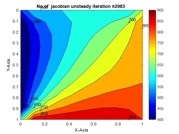
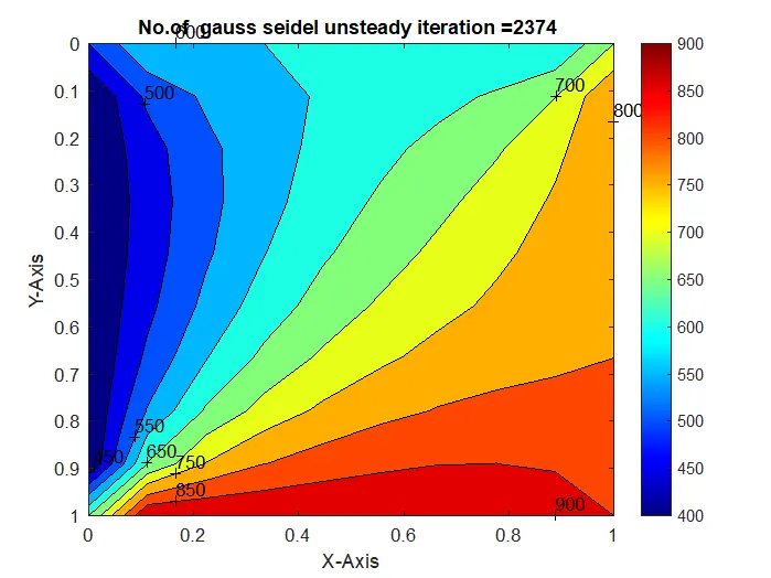
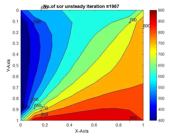
Result:
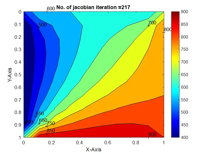
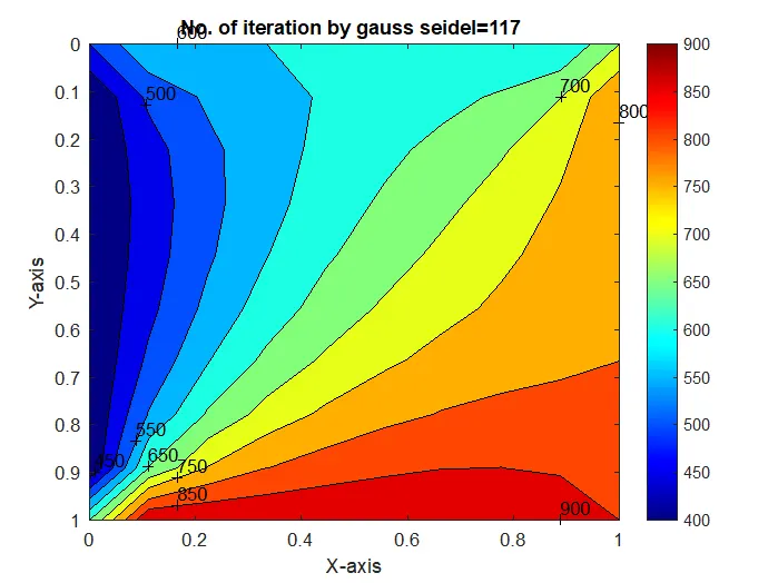
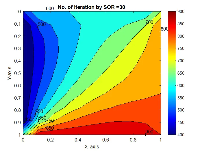
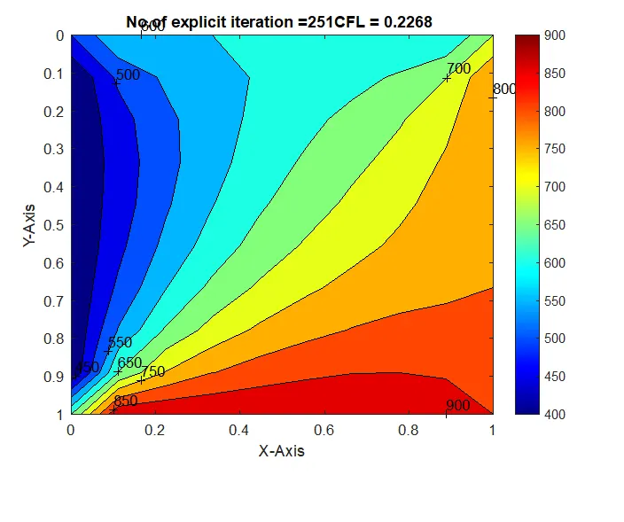
From the above program, We have found out No . of iteration required for the solution to be converge for different states.
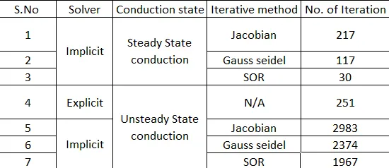
- Evidently with the use of Scaling factor omega in SOR method, the solution converged faster with lesser no. of iteration.
- Steady state has lesser no. of iteration,When compared to unsteady state of heat conduction.
- Explicit solution is a stable solution because it has a CFL value lesser than 0.5.