Deriving 4th order approximation of a 2nd order derivative using Taylor Table method
Aim:
To derive a 4th order approximation of a 2nd order derivative using Taylor's table.
* Central differencing, Skewed right-sided differencing, Skewed left-sided differencing.
* By using the coefficient obtained from the above scheme and to write a program in Matlab to evaluate the second-order derivative of the analytical function exp(x)*cos(x) and to compare it with the 3 numerical approximations.
- Central differencing:
No.of unknowns = Order of derivate+order of approximation -1
= 2+4-1
= 5.
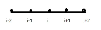
Δx^2⋅(∂^2u/∂^2x)=af(i-2)+bf(i-1)+cf(i)+df(i+1)+ef(i+2)
By using Taylor's series expansion, we will get
| Talyor's series expansion | |||||||
| f(i) | Δx.f'(i) | (Δx)^2.f''(i) | (Δx)^3.f'''(i) | (Δx)^4.f^iv(i) | (Δx)^5.f^v(i) | ||
| Stencils | af(i-2) | a | -2a | 4/2a | -8a/6 | 16a/24 | -32a/120 |
| bf(i-1) | b | -b | -b/2 | -b/6 | -b/24 | -b/120 | |
| cf(i) | c | 0 | 0 | 0 | 0 | 0 | |
| df(i+1) | d | d | d/2 | d/6 | d/24 | d/120 | |
| ef(i+2) | e | 2e | 4/2*e | 8/6*e | 16/24*e | 32e/120 | |
| ∑ | 0 | 0 | 1 | 0 | 0 | 0 | |
Converting the above table in a matrix form to find the unknowns:
clear all
close all
clc

A=[1 1 1 1 1;-2 -1 0 1 2; 4/2 1/2 0 1/2 4/2;-8/6 -1/6 0 1/6 8/6;16/24 -1/24 0 1/24 16/24];

B=[0;0;1;0;0];

X=inv(A)*B;
Solution:
A =

    1.0000    1.0000    1.0000    1.0000    1.0000
   -2.0000   -1.0000         0    1.0000    2.0000
    2.0000    0.5000         0    0.5000    2.0000
   -1.3333   -0.1667         0    0.1667    1.3333
    0.6667   -0.0417         0    0.0417    0.6667


B =

     0
     0
     1
     0
     0


X =

    0.0000
    1.0000
   -2.0000
    1.0000
    0.0000

>>
therefore a=0;b=1.0000;c=-2.0000;d=1.0000;e=0.0000
Matrix inversion is used to find the unknows
(∂^2u/∂^2x)=(af(i-2)+bf(i-1)+cf(i)+df(i+1)+ef(i+2))/Δx^2
substituting the unknows in the equation
(∂^2u/∂^2x)=(0f(i-2)+1.0000f(i-1)+1.0000f(i)+df(i+1)+0.0000f(i+2))/(Δx^2)
- Skewed right-sided differencing:
No.of unknowns = Order of derivate+order of approximation
= 2+4
= 6.
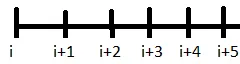
Δx^2⋅(∂^2u/∂^2x)=af(i)+bf(i+1)+cf(i+2)+df(i+3)+ef(i+4)+gf(i+5)
By using Taylor's series expansion, we will get
| Talyor's series expansion | |||||||
| f(i) | Δx.f'(i) | (Δx)^2.f''(i) | (Δx)^3.f'''(i) | (Δx)^4.f^iv(i) | (Δx)^5.f^v(i) | ||
| Stencils | af(i) | a | 0 | 0 | 0 | 0 | 0 |
| bf(i+1) | b | b | b/2 | b/6 | b/24 | b/120 | |
| cf(i+2) | c | 2c | 2c | 8c/6 | 16c/24 | 32c/120 | |
| df(i+3) | d | 3d | 9d/2 | 27d/6 | 81d/24 | 243d/120 | |
| ef(i+4) | e | 4e | 16e/2 | 64e/6 | 256e/24 | 1024e/120 | |
| gf(i+5) | g | 5g | 25g/2 | 125g/6 | 625g/24 | 3125g/120 | |
| ∑ | 0 | 0 | 1 | 0 | 0 | 0 | |
Converting the above table in a matrix form to find the unknowns:
clear all
close all
clc

A=[1 1 1 1 1 1;0 1 2 3 4 5;0 1/2 4/2 9/2 16/2 25/2;0 1/6 8/6 27/6 64/6 125/6;0 1/24 16/24 81/24 256/24 625/24;0 1/120 32/120 243/120 1024/120 3125/120];

B=[0;0;1;0;0;0];

X=inv(A)*B;
Solution:
A =

    1.0000    1.0000    1.0000    1.0000    1.0000    1.0000
         0    1.0000    2.0000    3.0000    4.0000    5.0000
         0    0.5000    2.0000    4.5000    8.0000   12.5000
         0    0.1667    1.3333    4.5000   10.6667   20.8333
         0    0.0417    0.6667    3.3750   10.6667   26.0417
         0    0.0083    0.2667    2.0250    8.5333   26.0417


B =

     0
     0
     1
     0
     0
     0


X =

    3.7500
  -12.8333
   17.8333
  -13.0000
    5.0833
   -0.8333
therefore a=3.7500;b=-12.8333;c=17.8333;d=-13.0000;e=5.0833;g=-0.8333.
Δx^2⋅(∂^2u/∂^2x)=af(i)+bf(i+1)+cf(i+2)+df(i+3)+ef(i+4)+gf(i+5)
(∂^2u/∂^2x)=(3.7500f(i)-12.8333f(i+1)+17.8333f(i+2)-13.000f(i+3)+5.0833f(i+4)+-0.8333f(i+5))/Δx^2⋅
- Skewed left-sided differencing:
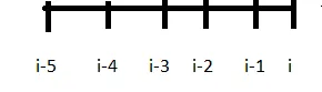
No.of unknowns = Order of derivate+order of approximation
= 2+4
= 6.
Δx^2⋅(∂^2u/∂^2x)=af(i)+bf(i-1)+cf(i-2)+df(i-3)+ef(i-4)+gf(i-5)
By using Taylor's series expansion, we will get
| Talyor's series expansion | |||||||
| f(i) | Δx.f'(i) | (Δx)^2.f''(i) | (Δx)^3.f'''(i) | (Δx)^4.f^iv(i) | (Δx)^5.f^v(i) | ||
| Stencils | af(i) | a | 0 | 0 | 0 | 0 | 0 |
| bf(i+1) | b | -b | b/2 | -b/6 | b/24 | -b/120 | |
| cf(i+2) | c | -2c | 2c | -8c/6 | 16c/24 | -32c/120 | |
| df(i+3) | d | -3d | 9d/2 | -27d/6 | 81d/24 | -243d/120 | |
| ef(i+4) | e | -4e | 16e/2 | -64e/6 | 256e/24 | -1024e/120 | |
| gf(i+5) | g | -5g | 25g/2 | -125g/6 | 625g/24 | -3125g/120 | |
| ∑ | 0 | 0 | 1 | 0 | 0 | 0 | |
Converting the above table in a matrix form to find the unknowns:
clear all
close all
clc

A=[1 1 1 1 1 1;0 -1 -2 -3 -4 -5;0 1/2 4/2 9/2 16/2 25/2;0 -1/6 -8/6 -27/6 -64/6 -125/6;0 1/24 16/24 81/24 256/24 625/24;0 -1/120 -32/120 -243/120 -1024/120 -3125/120];

B=[0;0;1;0;0;0];

X=inv(A)*B;
Solution:
X =

    3.7500
  -12.8333
   17.8333
  -13.0000
    5.0833
   -0.8333
therefore a=3.7500;b=-12.8333;c=17.8333;d=-13.0000;e=5.0833;g=-0.8333.
Δx^2⋅(∂^2u/∂^2x)=af(i)+bf(i-1)+cf(i-2)+df(i-3)+ef(i-4)+gf(i-5)
(∂^2u/∂^2x)=(3.7500f(i)-12.8333f(i-1)+17.8333f(i+2)-13.000f(i-3)+5.0833f(i-4)+-0.8333f(i-5))/Δx^2⋅
From the above images we have found out the coefficients of Central differencing,skew-left sided differencing,skew-right-sided differencing by Taylor's table method.
Given:
Analytical derivative=exp(x)*cos(x).
f(x)=exp(x)cosx
using uv formula
f'(x)= exp(x)cosx-exp(x)sinx
f''(x)=-2exp(x)sinx
Numerical derivative:
taking varying dx= linspace(pi/30,pi/300,20)
Program:
clear all
close all
clc

% analytical derivative
    %f(x)=exp(x)cosx
    %using uv formula
    %f'(x)= exp(x)cosx-exp(x)sinx
    %f''(x)=-2exp(x)sinx

%inputs
x= pi/5;
analytical_derivative = -2*exp(x)*sin(x);

% Central differencing
A=[1 1 1 1 1;-2 -1 0 1 2; 2 1/2 0 1/2 2;-8/6 -1/6 0 1/6 8/6;16/24 1/24 0 1/24 16/24];
B=[0;0;1;0;0];
C=inv(A)*B;


%Skewed right sided differencing
D=[1 1 1 1 1 1;0 1 2 3 4 5;0 1/2 4/2 9/2 16/2 25/2;0 1/6 8/6 27/6 64/6 125/6;0 1/24 16/24 81/24 256/24 625/24;0 1/120 32/120 243/120 1024/120 3125/120];
E=[0;0;1;0;0;0];
F=inv(D)*E;


% Skewed left-sided differencing:
G=[1 1 1 1 1 1;0 -1 -2 -3 -4 -5;0 1/2 4/2 9/2 16/2 25/2;0 -1/6 -8/6 -27/6 -64/6 -125/6;0 1/24 16/24 81/24 256/24 625/24;0 -1/120 -32/120 -243/120 -1024/120 -3125/120];
H=[0;0;1;0;0;0];
I=inv(G)*H;

%Numerical derivative
dx=linspace(pi/30,pi/300,20);

for i=1:length(dx)
left_skewed_scheme(i) = (I(1)*exp(x)*cos(x) + I(2)*exp(x-dx(i))*cos(x-dx(i))+I(3)*exp(x-2*dx(i))*cos(x-2*dx(i))+I(4)*exp(x-3*dx(i))*cos(x-3*dx(i))+I(5)*exp(x-4*dx(i))*cos(x-4*dx(i))+I(6)*exp(x-5*dx(i))*cos(x-5*dx(i)))/dx(i)^2;
right_skewed_scheme(i)  = (F(1)*exp(x)*cos(x) + F(2)*exp(x+dx(i))*cos(x+dx(i))+F(3)*exp(x+2*dx(i))*cos(x+2*dx(i))+F(4)*exp(x+3*dx(i))*cos(x+3*dx(i))+F(5)*exp(x+4*dx(i))*cos(x+4*dx(i))+F(6)*exp(x+5*dx(i))*cos(x+5*dx(i)))/dx(i)^2;
central_differencing(i) = (C(1)*exp(x-2*dx(i))*cos(x-2*dx(i))+C(2)*exp(x-dx(i))*cos(x-dx(i))+C(3)*exp(x)*cos(x)+C(4)*exp(x+dx(i))*cos(x+dx(i))+C(5)*exp(x+2*dx(i))*cos(x+2*dx(i)))/dx(i)^2;
end

error_left = abs(left_skewed_scheme-analytical_derivative);
error_right = abs(right_skewed_scheme-analytical_derivative);
error_central = abs(central_differencing-analytical_derivative);

loglog(dx,error_left,'r',dx,error_right,'b',dx,error_central,'g')
xlabel('dx');
ylabel('Error of the scheme');
legend('left skewed scheme','right skewed scheme','Central differencing');
grid on
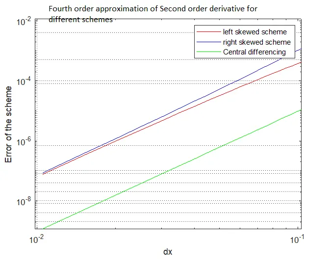
Graph:
Result:
From the above graph,We can say that
*Fourth order approximation of second derivative - Central differencing has least error when other to others,hence it has more accuracy because it takes information from both sides symmentrically.
* In CDS cannot be applied at boundary condition because unavailablity of Nodes at both sides symmentrically,so skewed scheme is applied at boundaries.