Week 9 - FVM Literature Review
*AIM:-
-Define Finite volume method(FVM)
-Write down the difference between FVM and FDM.
-describe the need for interpolation schemes and flux limiters in FVM, use the 1D linear heat conduction equation as an example.
*Objectives:-
-Define Finite volume method, Also define difference between FVM & FDM.
- Consider example of 1-D heat condution equation to describe how to solve FVM problem.
-Explain about grid generation process in FVM.
-Describe how to discretize the equation by using various interpolation method.
-Calculate the solutions for discretize equations.
- Compare calculated numerical method with actual results.
*Finite volume method(FVM):-
-The finite volume method is a discretization technique for the approximation of single or system of partial differential equations expressing the conservation, or balance of one or more quantities.
-These partial differential equations are oftain called the conservations law. They describes the relation between partial derivative of unknown field such as temperature, concentration, pressure, molar fraction, density of eletrons or probability density function, with respect to variables within the domain under consideration.
-Therefore, FVM is used by various numerical techniques in which the solution is descretised in to the number of control volumes over which integrals of conservation laws are directly discretised.
*Difference between FVM and FDM:-
1) Finite difference method(FDM):-
-It is created from basic definition of differentiation that
-FDM is very simple method compare to FVM.
-It is easy method but not reliable for conservative differential equations and solution having shocks.
-Extending to higher order accuracy is very simpke.
-In FDM discretization is based on differential form of the PDE's to be solve. It derivative is replaced with an approximate difference formula, that can be generally derived by taylor series expansion.
-The computational domain is generally devided in to hexahedral cells, and solution will be obtained at nodal points.
-The FDM is easiest to understand when the physical grid is cartesian. We can not implement this method, when grids are not allign in x,y or z direction.
-The discretization result in a system of equation of the variables at nodal points, and once the solution is found , then we have discrete representation of solution.
2) Finite volume method:-
-It is a numerical tool that is borrowed from calculus of variation. here we assume that some trial function and multiply that trial function with weighting function.
-Then this weighting function is multiplied with trial function then integrated over the control volume and equated to zero. Then we get one set of algebric equations. solving that will give solution.
-In FVM discretization is based upon the integral form of PDE to be solved.(eg. conservation of mass, momentum and energy). The PDE is written in form which can be solved for the given finite volume.
-The computational domain is discretized in to finite volume and then for every volume the governing equations are solve.
-The resulting system of equation ussually involves fluxes of conserved variable, and thus the calculation of fluxes is very important in FVM.
-The basic advantage of this method over FDM is it does not require the use of structured grid, and effort to convert the given mesh in to structured numerical grid internally is completely avoided.
-As with FDM , the resulting approximated solution is a discrete, but the variables are typically placed at cell centres rather than at nodal points. This is not always true. There are also face- centered finite volume method.
*Problem statement:-
-The governing equation for 1-D linear heat condution equation is
`d/dx (k (dT)/dx)+q=0`
Where, k= Thermal conductivity
T= Temperature
dx= Control volume
q= Heat generation in the system
*Initial condition & Boundary condition:-
-The initilal and boundary condition is a most important requirement for any simulation.
-In this case initial and boudary conditions are:-
Plate thickness(L)= 0.02 mm
Thermal conductivity(k)= 0.5 w/m.k
Heat generation(q)= 1000e3 kw/m^3
Temperature at point A(Ta)=100
Temperature at point B(Tb) =200
Area (A)=1
*Finite volume interpolation scheme:-
-In the field of numerical analysis interpolation is the time of estimation, a method of constructing new data points within the range of discrete set of known data point.
- The approximation of surface and volume integrals may require values of variables at locations other than the computational nodes of the control volumes i.e. to evaluate temperature value and temperature gradient we are going to use interpolation technique through the nodal value.
- These interpolation scheme are not so different from taylor series expansion in Finite difference method. Only difference is in the FVM differentials need to be evaluate on the over all control volume rather than nodal points.
* Following are the varoius interpolation scheme for different orders:-
1) First order upwind difference scheme (UD)
2) Central difference scheme (CD)
3) Second order upwind or linear upwind differencing (LUD) scheme
4) Quadratic upwind interpolation (QUICK)
5) Total variation diminishing (TVD) scheme
1) First order upwind difference scheme (UD):-
- As a name suggest it is the first order accurate simplest numerical scheme, where value at the interface assume same as the value at center of the control volume depending upon the flow direction.
- The interpolation scheme is equvivalent to using forward or backward difference approximation (depending on flow direction) which gives stable calculation but its very diffusive.
`((∂∅)/(∂x))_p=(∅_E-∅_p)/(∆x)`
-Since it uses values at point E and P to evaluate the gradient `((∂∅)/(∂x))` at p, The formula is called forward differencing.
-Similary for backward differencing `((∂∅)/(∂x))` at p will be
`((∂∅)/(∂x))_p=(∅_P-∅_W)/(∆x)`
-By using first order upwind scheme, we will get
`(kA (dT)/dx)_e=k_e A((T_E-T_P)/(∂x))`
`(kA (dT)/dx)_w=k_w A((T_P-T_W)/(∂x))`
-After put in the equation we will get
`[k_e A((T_E-T_P)/(∂x))-k_w A((T_P-T_W)/(∂x))]+qA∂x=0`
2) Central difference scheme (CD):-
- It is the second order accurate approximation scheme in which value of flux is defined by linear interpolation amid the center of the control volume.
`((∂∅)/(∂x))_p=(∅_E-∅_W)/(2∆x)`
- Above equation use value at E and W to evaluate the gradient at the mid-point p, and is called central difference formula.
- The quadratic dependence of the error on grid spacing means that after grid refinment the error reduces more quickly in a second order accurate difference scheme than in the first order accurate.
- By using central difference scheme, we will get
`(kA (dT)/dx)_e=k_e A((T_E-T_P)/(2∂x))`
`(kA (dT)/dx)_w=k_w A((T_P-T_W)/(2∂x))`
-After put in equation we will get
`[k_e A((T_E-T_P)/(2∂x))-k_w A((T_P-T_W)/(2∂x))]+qA∂x=0`
3) Second order upwind or linear upwind differencing (LUD) scheme :-
- The spatial accuracy of the first order scheme can be improves by including 3 data points instead of just 2, which offers the more accurate finite difference stencil for approximation of spetial derivative
`((∂∅)/(∂x))_p=(3∅_E-∅_W)/(2∆x)`
-by using linear upwind differencing scheme, we will get
`(kA (dT)/dx)_e=k_e A((3T_E-T_P)/(2∂x))`
`(kA (dT)/dx)_w=k_w A((3T_P-T_W)/(2∂x))`
-This cheme is less diffusive compare to first order accurate scheme and is called linear upwind scheme.
-After put in equation we will get
`[k_e A((3T_E-T_P)/(2∂x))-k_w A((3T_P-T_W)/(2∂x))]+qA∂x=0`
4) Quadratic upwind interpolation (QUICK):-
- It is derived using polynomial fitting. It is relatively straight forward to demostrate the third order accuracy of the quick differencing scheme for the convective flux at a midpoint cell face in uniform grid of spacing delta x.
- The QUICK scheme calculates the value phi_e at the east cell face of general node as
`∅_e=3/8 ∅_E+6/8 ∅_P-1/8 ∅_W`
`(kA (dT)/dx)_e=k_e A((3/8 T_E+6/8 T_P-1/8 T_W)/(∂x))`
`(kA (dT)/dx)_w=k_w A((3/8 T_E+6/8 T_P-1/8 T_W)/((∂x)/2))`
-After put in equation we will get
`[k_e A((3/8 T_E+6/8 T_P-1/8 T_W)/(∂x))-k_w A((3/8 T_E+6/8 T_P-1/8 T_W)/(∂x))]+qA∂x=0`
5) Total variation diminishing (TVD) scheme:-
- Scheme of third order and above have been developed for the discretization of convective terms with varying degree of success.
-Implementation of boundary conditions can be problematic with such higher order scheme. The facts that QUICK scheme and higher order schemes can give.
-Undershoots and overshoots has led to the development of second order schemes that avoid these problems.
-The class of TVD (total variation diminishing) schemes has been specially formulated to achieve oscillation- free solutions and has proved to be useful in the CFD calculations.
-The general form of the east face value phi_e within a discretisation scheme may be written as
`∅_e=∅_p+1/2 Ѱ(r)(∅_E-∅_p)`
*THE function of psi for various discretisation scheme:-
1) For the UD scheme `Ѱ(r)=0`
2) For the CD scheme `Ѱ(r)=1`
3) For the LUD scheme `Ѱ(r)=r`
4) For the QUICK scheme `Ѱ(r)=(3+r)/(4)`
*Program:-
clear all
close all
clc

%Plate thickness in mm
L=0.02;
%Thermal conductivity in W/m*k
k=0.5;
%Heat generation in KW/m^3
q=1000e3;

%Initial temperature at point A
Ta=100;
%Initial temperature at point B
Tb=200;

%Area
A=1;

%Grid generation
%Devided by 5 volumes
nx=5;
dx=L/nx;
%Specify center node of each volume
x=dx/2:dx:L-(dx/2);

%Defining matrix size according to the nx
LHS=zeros(nx,nx);
RHS=zeros(nx,1);

%Apply first order upwind scheme (Between point A and B)
for i=2:nx-1
    LHS(i,i)=2*(k*A)/dx;
    LHS(i,i-1)=-(k*A)/dx;
    LHS(i,i+1)=-(k*A)/dx;
    RHS(i)=q*A*dx;
end

%At A point
LHS(1,1)=3*(k*A)/dx;
LHS(1,2)=-(k*A)/dx;
RHS(1)=2*(k*A*Ta)/dx+q*A*dx;

%At B point
LHS(end,end)=3*(k*A)/dx;
LHS(end,end-1)=-(k*A)/dx;
RHS(end)=2*(k*A*Tb)/dx+q*A*dx;

%Rearranging matrices to calculate temperature matrix
T=LHS^-1*RHS;
x_an=linspace(0,L,100);
T_an=((Tb-Ta)/L+(q/(2*k))*(L-x_an)).*x_an+Ta;


%plotting
plot(x_an*100,T_an)
hold on
plot(x*100,T,':*','markerfacecolor','g','color','r')
grid on
axis([0 2 90 280]);
title('comperision of numerical and analytical method');
xlabel('length in cm');
ylabel('temperature');
legend('analytical solution','numerical solution');

%Error
T_an_pt=((Tb-Ta)/L+(q/(2*k))*(L-x)).*x+Ta;
error=max(abs(T'-T_an_pt))
*Results:-
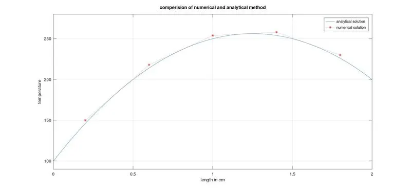
-Above figure exhibits the temperature value calculated for plate which have thickness 2 cm with both analytical and numerical method.
-We can see, even with a coarse grid of 5 nodes, the agreement is very good.
-Increase the accuracy by incresing the number of grid within length L.
* Error:-
-It find out using the difference between temperature calculated by analytical method and numerical method.
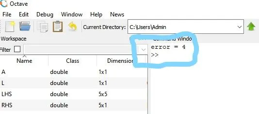
-So error for our numerical solution of 5 control volume is 4.
-we can reduce it by making grid fine.