Week 9 - FVM Literature Review
DESCRIPTION:
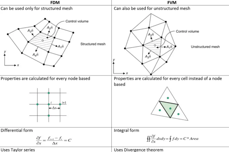
1.To understand the major differences between Finite Difference Method (FDM) and Finite Volume Method (FVM)
2.To describe the need for interpolation schemes and flux limiters in FVM using 1D linear heat conduction equation.
ANSWER:
There are 3 ways to solve numerical problems in computational fluid dynamics (CFD)
- Finite Difference Method
- Finite Element Method
- Finite Volume Method
Finite Difference Method
Finite difference methods are a class of numerical methods invloving the discretisation of spatial domain (broken into a finite number of steps)
and the value at these discrete points is solved using equations with finite differences and values from its neighbouring points.
boundary conditions are needed to to truncate the computational domain.THey represent communication with the surrounding world.With the finite difference method,we can easily run computation problems handling with boundary conditions.
The FDM method is typically defines into hexahedral cells and the solution is always obtained at a nodal point or nodes.Regular grids are useful for every large scale simulations.
The finite difference method is difficult to use in complex or irregular shapes and products.
This is because it does not lend itself for local grid refinement or anything similar to an adaptive mesh.
If one can overcome the boundary condition problem on the curved boundaries,the method gives very efficient and high quality results.
The finite difference method is defined as dimension per dimension,which increases the element order for getting more accurate values.
Finite Volume Method
It is similar to finite difference method i.e that a model is divided into small and finite elements of geometrically similar shapes.These are called cells.
It is based upon the integral form of PDE to be solved like mass,momentum conservation. The PDE is initially written so as to solve one cell or a finite volume. The computational domain is discretised into finite volumes and then the governing equations are solved (for every volume).
The calculation of fluxes is very important in the finite volume method as the resulting system of equations involves the fluxes of the conserved variable.
Since it only calculates the flux calculation at the boundaries,it also solves non-linear problems.
The accuracy of the finite volume method can be increased by refining the mesh around the corner.But the functions that approximate the solution when using FVM cannot easily made of higher order.
The major advantage in FVM is that there is no requirement of using the structural grids and the effort to convert the mesh into structured njumerical grid internally can be avoided.
As with FDM,the resulting solution is discrete, but the variables are typically placed at centres rather than at nodal points.
FVM guarantee the local and global conservation of the system.
Now consider the 1-D heat conduction equation
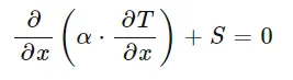
where S=source term and
α=thermal Diffusivity
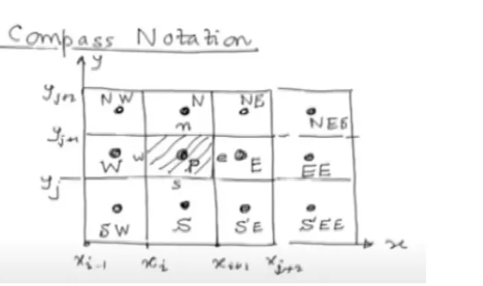
Consider the control volume P and the centroid at P as in the figure.
The figure has a set of control volume with the centroids located at P,E(East),W(West),N(North),S(South) and the further point with representation.
Coming back to the 1-D heat conduction equation,because of being one dimensional it does not have a north and south control volume.Consider a small volume dv in the control volume P,the integral form of the equation for the small volume is
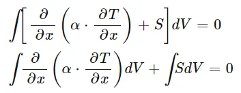
Now as dV=A.dx,

On solving the equation,

Savg,α are the function of temperature.We need to linearise it.
Now assuming that α is a constant

(Heat flux out)-(heat flux in)+(source term)=0
Need for interpolation schemes:
To calculate the Tw and Te, the temperatures at the west and east faces,we have the value at Tp,Te and Tw by interpolating the values,we can get the temperature at the east and west faces.By using them we can calculate the thermal diffusivity of the faces are αe and αw.There are different ways of interpolation.Some of the ways are given by
- Upwind interpolation scheme.
- Linear interpolation scheme.
- Quadratic Interpolation Scheme.
Upwind interpolation scheme
The upwind interpolation scheme is used for approximating the value of a variable at either front or back face of the control volume which is given by
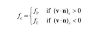
The interpolation scheme is eqivalent to using a backward or forward finite difference approximation (depending on the direction of the flow).It is the first order accurate schem and is numerically diffusice with a coefficient of numerical diffusion.
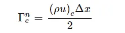
The scheme is developed from the convective flows with the suppressed diffusion effects.
LInear interpolation scheme
The value of the variable at the control volume face center approximate from the values near two computational nodes.This location at 'e' on a cartesian grid,the variable value is approximated by
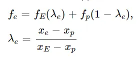
The linear interpolation is equivalent to the use of the central differencing formula of the first order derivative, and hence, this is also termed as the central differencing scheme.This scheme is second derivative accurate and may oroduce an oscillary solution.
Quadratic upwind interpolation
A quadratic interpolation is the three order scheme, it is derived from the poltnomial fitting.It is also represented as the QUICk interpolatin.The quick interpolation on a uniform cartesian grid is given by,

where D,U and UU denote the downstream,the first upstream and the second upstream node respectively.
Quick scheme is prone to oscillation because of the 3rd order.
Flux Limiter
In solving the convective flow fields, it is observed that in the discontinuity for the higher order, it is observed that the oscillation is more and the solution becomes more stable due to this reason.
To obtain the highly accurate and oscillation free results we need to use the flux limiter function.
The function provides the smooth region over the flow and maintains the first order accuracy.Flux limiets are mainly used to get the total variation diminshing.
Their simple forms for !D equation are given by

This terms represent edge fluxes for the ith cell.
Where,fluxes can be represented by low and high resolution schemes.
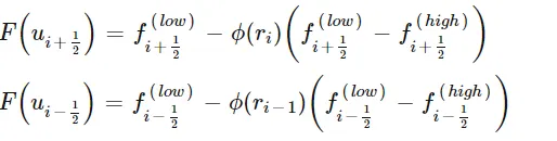
where
f low=low resolution flux
f high=high resolution flux
ϕ(r)=flux limiter function
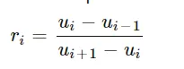
where r represents the ratio of succesive gradients on the solution mesh
the liniter function is constrained to be greater than or equal to zero
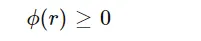
when the limiter equals to zero, the flux represents the low resolution scheme.
when the limiter equals to one, the flux represents the low resolution scheme.
There are many limiters having distinguished characters and are seleted according to the problem.There is no particular limiter found to work well for all and it is selected by the trial and error method.