Week 5 - Mid term project - Solving the steady and unsteady 2D heat conduction problem
DESCRIPTION:
To solve a given 2d heat conduction equation using 3 methods (Jacobian,gauss and succesive over-relaxation technique) for both steady and unsteady conditions.
The given 2d heat conduction equation is
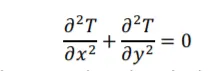
Here we assume that the no:of elements in x axis is equal to the no: of elements in the y axis
i.e nx=ny
therefore we get △x^2=△y^2
Now Solving for this equation when we assume that the equation is a steady state equation
MAIN CODE:
clear all
close all
clc
%initialising the variables and the arrays
l=1;
nx=ny=30;
x=linspace(0,l,nx);
y=linspace(0,l,ny);
dx=x(2)-x(1);
dy=y(2)-y(1);
error=9e9;
tol=1e-4;
Tl=400;
Tt=600;
Tr=800;
Tb=900;
T1=ones(nx,ny);
%for sqr boundary
alpha=1.84;

%Assigning values to boundary
T1(2:ny,1)=Tl;
T1(2:ny,nx)=Tr;
T1(1,2:nx)=Tt;
T1(ny,2:nx)=Tb;

%calculating the corner variables by taking the average
T1(1,1)=(Tt+Tl)/2;
T1(nx,1)=(Tb+Tl)/2;
T1(nx,ny)=(Tb+Tr)/2;
T1(1,ny)=(Tt+Tr)/2;
[X,Y]=meshgrid(x,y);
Told1=T1;
Told2=T1;
Told3=T1;
T2=T1;
T3=T1;
iteration_no=1;
iterative_solver=1;
a=(dx^2)+(dy^2)/((dx*dy)^2);
b=2*a;
k=b/((dx^2)*(dy^2));
t1=1;
%jacobian method for 2 dimension
tic
for iterative_solver=1;

  if iterative_solver==1
    while(error>tol)
    for i=2:nx-1
      for j=2:ny-1
        t1=(Told1(i-1,j)+Told1(i+1,j));
        t2=(Told1(i,j-1)+Told1(i,j+1));
        T1(i,j)=0.25*(t1+t2);


      end
    end
    error=max(max(abs(Told1-T1)));
    Told1=T1;
    iteration_no=iteration_no+1;

   end
  end
%plotting jacobian_2d
  figure(1)
  [M,N]=contourf(X,Y,T1);
  clabel(M,N)
  colormap(jet)
  colorbar
  text=sprintf("Steady iteration no: for jacobi method=%d",iteration_no);
  title(text);
  xlabel("X axis","fontsize",24)
  ylabel("Y axis","fontsize",24)
  pause(50)
end
time1=toc;


%gauss2d
error=9e9;
tic
for iterative_solver=2;
  iteration_no=1;
  if iterative_solver==2
    while(error>tol)
    for i=2:nx-1
      for j=2:ny-1
        t1=(T2(i-1,j)+Told2(i+1,j));
        t2=(T2(i,j-1)+Told2(i,j+1));
        T2(i,j)=0.25*(t1+t2);


      end
    end
    error=max(max(abs(Told2-T2)));
    Told2=T2;
    iteration_no=iteration_no+1;

   end
  end
  %plotting gauss_method_2d
  figure(2)
  [M,N]=contourf(X,Y,T2);
  clabel(M,N)
  colormap(jet)
  colorbar
  text=sprintf("Steady iteration no: for Gauss method=%d",iteration_no);
  title(text);
  xlabel("X axis","fontsize",24)
  ylabel("Y axis","fontsize",24)
  pause(50)
end
time2=toc;


%solving sor
error=9e9;
tic
for iterative_solver=3;
  iteration_no=1;
  if iterative_solver==3
    while(error>tol)
    for i=2:nx-1
      for j=2:ny-1
        T3(i,j)=(((1-alpha)*Told3(i,j))+(0.25*alpha*((T3(i-1,j)+Told3(i+1,j))+(T3(i,j-1)+Told3(i,j+1)))));
      end
    end
    error=max(max(abs(Told3-T3)));
    Told3=T3;
    iteration_no=iteration_no+1;

   end
  end
  %plotting sor_2d
  figure(3)
  [M,N]=contourf(X,Y,T3);
  clabel(M,N)
  colormap(jet)
  colorbar
  text=sprintf("Steady iteration no: for sor method=%d",iteration_no);
  title(text);
  xlabel("X axis","fontsize",24)
  ylabel("Y axis","fontsize",24)
  pause(50)
end
time3=toc;
OUTPUT:
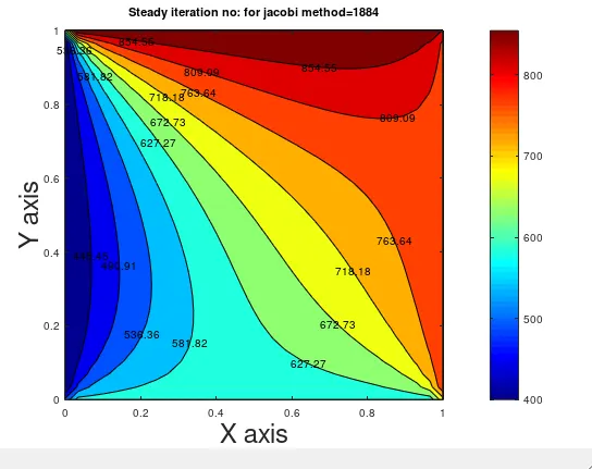
1) For the jacobian method it took a time of t=150.53s
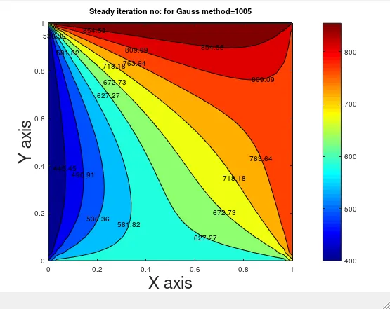
2)For gauss method it took a time t=113.07s
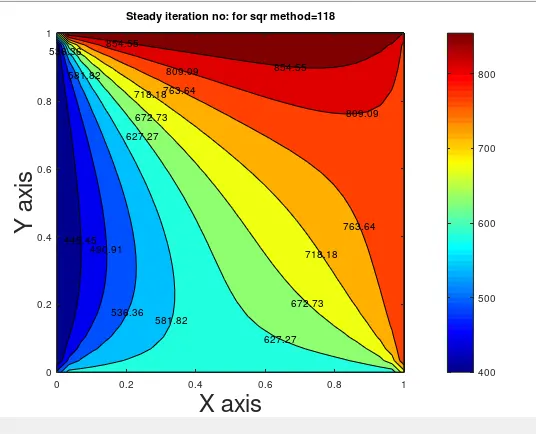
3) and for succesive over relaxation method, it took a time t=58.02s
Unsteady Flow
In Unsteady flow the generalised 2 dimensional heat equation becomes
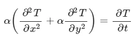
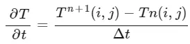
When discretising the above equation using central differencing with respect to x and y, we get


The time equation is discretised using forward differencing
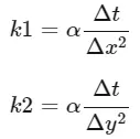
The 2 constants k1 and k2 is calculated using the formula
Assuming nx=ny such that △x^2=△y^2,we get the equation

Solving unsteady flow(Explicit):
clear all
close all
clc

%initialising the variables and the arrays
l=1;
nx=ny=30;
x=linspace(0,l,nx);
y=linspace(0,l,ny);
dx=x(2)-x(1);
dy=y(2)-y(1);
dt=0.01;
error=9e9;
tol=1e-4;
Tl=400;
Tt=600;
Tr=800;
Tb=900;
T1=ones(nx,ny);
%for sqr boundary
alpha=0.015;


%Assigning values to boundary
T1(2:ny,1)=Tl;
T1(2:ny,nx)=Tr;
T1(1,2:nx)=Tt;
T1(ny,2:nx)=Tb;

%calculating the corner variables by taking the average
T1(1,1)=(Tt+Tl)/2;
T1(nx,1)=(Tb+Tl)/2;
T1(nx,ny)=(Tb+Tr)/2;
T1(1,ny)=(Tt+Tr)/2;
[X,Y]=meshgrid(x,y);
Told1=T1;
iteration_no=1;
iterative_solver=1;

%factor k
k1=(alpha*dt)/(dx^2);
k2=(alpha*dt)/(dy^2);
[X,Y]=meshgrid(x,y);

%calculating 2d transient heat conduction state explicitly
tic
for iterative_solver=1;

  if iterative_solver==1
    while(error>tol)
    for i=2:nx-1
      for j=2:ny-1
        %t1=k1*(Told1(i+1,j)-2*Told1(i,j)+Told1(i-1,j));
        %t2=k2*(Told1(i,j+1)-2*Told1(i,j)+Told1(i,j-1));
        T1(i,j)=Told1(i,j)+(k1*(Told1(i+1,j)-2*Told1(i,j)+Told1(i-1,j)))+(k2*(Told1(i,j+1)-2*Told1(i,j)+Told1(i,j-1)));%+t1+t2;


      end
    end
    error=max(max(abs(Told1-T1)));
    Told1=T1;
    iteration_no=iteration_no+1;

   end
  end
  %plotting the transient equation
  figure(1)
  [M,N]=contourf(X,Y,T1);
  clabel(M,N)
  colormap(jet)
  colorbar
  text=sprintf("Steady iteration no: for explicit=%d",iteration_no);
  title(text);
  xlabel("X axis","fontsize",24)
  ylabel("Y axis","fontsize",24)
  pause(50)
end

time1=toc;
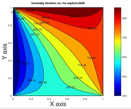
OUTPUT:
For explicit function,it took a time of 151.02s
Solving unsteady flow(implicit):
clear all
close all
clc

%initialising the variables and the arrays
l=1;
nx=ny=30;
x=linspace(0,l,nx);
y=linspace(0,l,ny);
dx=x(2)-x(1);
dy=y(2)-y(1);
dt=0.01;
error=9e9;
tol=1e-4;
Tl=400;
Tt=600;
Tr=800;
Tb=900;
%for sqr boundary
%alpha=1.4;

%Assigning values to boundary
T1(2:ny,1)=Tl;
T1(2:ny,nx)=Tr;
T1(1,2:nx)=Tt;
T1(ny,2:nx)=Tb;

%calculating the corner variables by taking the average
T1(1,1)=(Tt+Tl)/2;
T1(nx,1)=(Tb+Tl)/2;
T1(nx,ny)=(Tb+Tr)/2;
T1(1,ny)=(Tt+Tr)/2;
[X,Y]=meshgrid(x,y);
Told1=T1;
Told2=T1;
Told3=T1;
T2=T1;
T3=T1;
iteration_no=1;
iterative_solver=1;

Prev_Tdt1=Told1;
Prev_Tdt2=Told1;
Prev_Tdt3=Told1;

alpha=1.85;%for sor boundary
alpha1=25.5;

%factors k1 and k2
k1=(alpha1*dt)/(dx^2);
k2=(alpha1*dt)/(dy^2);

%jacobi iteration
term1=1/(1+2*k1+2*k2);
term2=k1*term1;
term3=k2*term1;
%jacobian method for 2 dimension
tic
for iterative_solver=1;

  if iterative_solver==1
    while(error>tol)
    for i=2:nx-1
      for j=2:ny-1
        t1=(Told1(i-1,j)+Told1(i+1,j));
        t2=(Told1(i,j-1)+Told1(i,j+1));
        T1(i,j)=term1+Prev_Tdt1(i,j)+(term2*t1)+(term3*t2);


      end
    end
    error=max(max(abs(Told1-T1)));
    Told1=T1;
    iteration_no=iteration_no+1;

   end
  end
%plotting jacobian_2d
  figure(1)
  [M,N]=contourf(X,Y,T1);
  clabel(M,N)
  colormap(jet)
  colorbar
  text=sprintf("Unsteady iteration no: for jacobi method=%d",iteration_no);
  title(text);
  xlabel("X axis","fontsize",24)
  ylabel("Y axis","fontsize",24)
  pause(50)
end
time1=toc;

%gauss2d
error=9e9;
tic
for iterative_solver=2;
  iteration_no=1;
  if iterative_solver==2
    while(error>tol)
    for i=2:nx-1
      for j=2:ny-1

        t1=(T2(i-1,j)+Told2(i+1,j));
        t2=(T2(i,j-1)+Told2(i,j+1));
        T2(i,j)=(term1*Prev_Tdt2(i,j))+((term2*t1)+(term3*t2));


      end
    end
    error=max(max(abs(Told2-T2)));
    Told2=T2;
    iteration_no=iteration_no+1;

   end
  end
  %plotting gauss_method_2d
  figure(2)
  [M,N]=contourf(X,Y,T2);
  clabel(M,N)
  colormap(jet)
  colorbar
  text=sprintf("Unsteady iteration no: for Gauss method=%d",iteration_no);
  title(text);
  xlabel("X axis","fontsize",24)
  ylabel("Y axis","fontsize",24)
  pause(50)
end
time2=toc;

%solving sor
error=9e9;
tic
for iterative_solver=3;
  iteration_no=1;
  if iterative_solver==3
    while(error>tol)
    for i=2:nx-1
      for j=2:ny-1
        %T3(i,j)=(((1-alpha)*Told3(i,j))+(0.25*alpha*((T3(i-1,j)+Told3(i+1,j))+(T3(i,j-1)+Told3(i,j+1)))));
        t1=(alpha*T3(i-1,j)+(1-alpha)*Told3(i-1,j)+Told3(i+1,j));
        t2=(alpha*T3(i,j-1)+(1-alpha)*Told3(i,j-1)+Told3(i,j+1));
        T3(i,j)=(Prev_Tdt3(i,j)*term1)+((term2*t1)+(term3*t2));

      end
    end
    error=max(max(abs(Told3-T3)));
    Told3=T3;
    iteration_no=iteration_no+1;

   end
  end
  %plotting sor_2d
  figure(3)
  [M,N]=contourf(X,Y,T3);
  clabel(M,N)
  colormap(jet)
  colorbar
  text=sprintf("Unsteady iteration no: for sor method=%d",iteration_no);
  title(text);
  xlabel("X axis","fontsize",24)
  ylabel("Y axis","fontsize",24)
  pause(50)
end
time3=toc;
OUTPUT:
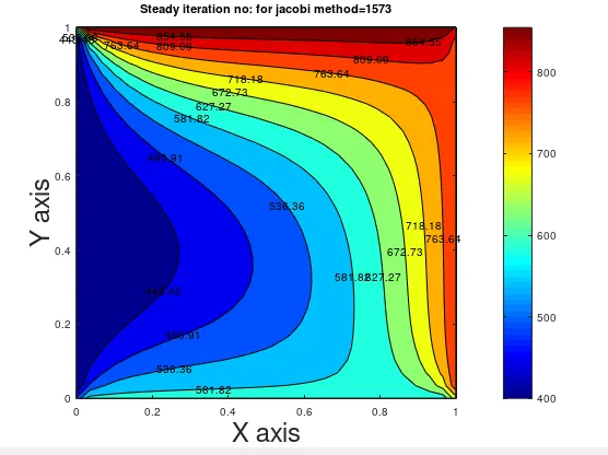
1)For jacobi iteration,it took a time of 231.17s
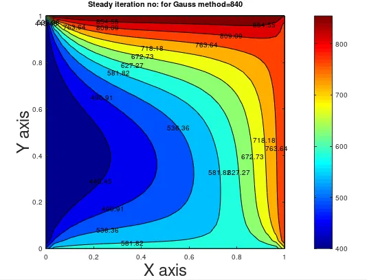
2)For gauss iteration,it took a time of 115.1s
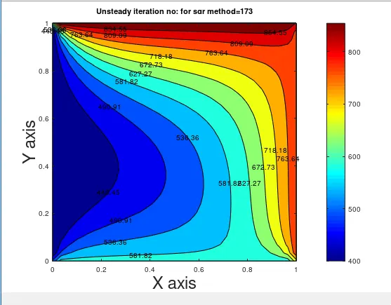
3) for sor method,it took a time of 68.273s
CONCLUSION:
1)FOR STEADY FLOW ITERATION:
| Method | No:of iterations | Time taken(s) | Error |
| Jacobi | 1884 | 150.53 | 9.9722e-5 |
| Gauss | 1005 | 113.07 | 9.9194e-5 |
| SOR | 115 | 52.02 | 8.8417e-5 |
2)FOR UNSTEADY FLOW ITERATION:
| Method | No: of iterations | Time taken(s) | Error |
| Jacobi | 1573 | 231.17 | 9.9636e-5 |
| Gauss | 840 | 115.10 | 9.7690e-5 |
| SOR | 173 | 68.273 | 9.6446e-5 |
From the above tabulations we can confirm that the successive over relaxation method converges towards the solution within a small time and few number of iterative cycles, thereby giving a minimum error value.
Therefoe the succesive over relaxation method is cost effective when compared to both jacobie and gauss method.