Week 9 - FVM Literature Review

AIM:

• To define finite volume method
• To write down the difference between FDM and FVM.
• To describe the need for interpolation schemes and the flux limiters in FVM.

FINITE VOLUME METHOD:

The finite volume method (FVM) is a method for representing and evaluating partial differential equations in the form of algebraic equations. In the finite volume method, volume integrals in a partial differential equation that contain a divergence term are converted to surface integrals, using the divergence theorem. These terms are then evaluated as fluxes at the surfaces of each finite volume. Because the flux entering a given volume is identical to that leaving the adjacent volume, these methods are conservative. Another advantage of the finite volume method is that it is easily formulated to allow for unstructured meshes. In contrast a finite volume method evaluates exact expressions for the average value of the solution over some volume, and uses this data to construct approximations of the solution within cells.

DIFFERENCE BETWEEN FDM AND FVM:

FINITE DIFFERENCE METHOD	FINITE VOLUME METHOD
Discretization is based on differential form of governing equation.	Discretization is based on integral form of governing equation.
The dependent variables are stored at regular grid points and derivatives are expressed in terms of differences between values on neighbouring grid points using expressions derived from truncating Taylor's series.	The domain of interest is divided into a large number of mesh, and the equations of interest are integrated over each cell. The assumption is that the dependent variables are constant over each cell (the value is usually stored at the cell centre).
This method can only be applied on simple geometries.	The cell can be any shape which allows much more complex geometries to be considered.
The discretization results in a system of equation of the variable at nodal points and once a solution is found then we have a discrete representation of the solution.	The discretization results in a system of equation of the variable at cell centre and if the nodal values are required it can be obtained by interpolation schemes.

INTERPOLATION SCHEMES:

The approximation of surface and volume integrals may require values of the variable at location other than the computational nodes of the control volume. Values at these locations are obtained using interpolation schemes.

Consider an example of 1D heat conduction equation

`del/(delx)(alpha(delT)/(delx))+s = 0`

Where,

            `alpha` is thermal diffusivity which depends on temperature at a point.so it is function of T.

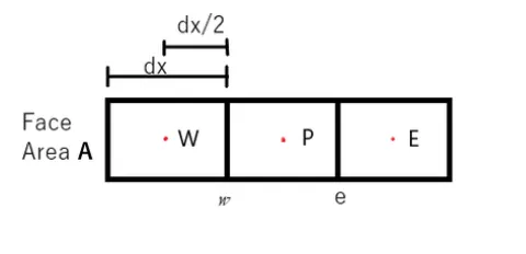
We consider P, W, E as the cell centres of the respective cells. To calculate the temperature at point P, we take information from the neighbouring cells W and E and it is called as gradient scheme.

`int(del/(delx)(alpha(delT)/(delx))+s)dV = 0`

`int(del/(delx)(alpha(delT)/(delx)))dV+intsdV = 0`

Since small volume is equal to area multiplied by dx.

`int(del/(delx)(alpha(delT)/(delx)))Adx+intsdV = 0`

after applying intergral limits we have,

`alphaA((delT)/(delx))_E - alphaA((delT)/(delx))_W +barS dV =0`

`alphaA((T_E -T_P)/(delx)) - alphaA((T_P-T_W)/(delx)) +barS dV =0`

by applying forward and backward differencing for east and west sides we got the above equation.

we know that alpha is function of T so the equation becomes,

`alpha_eA((T_E -T_P)/(delx)) - alpha_wA((T_P-T_W)/(delx)) +barS dV =0`

so we need the values of alpha_e and `alpha_w` for which we need `t_e` and`t_w` to get the value we use interpolation schemes. 

There are types of interpolation schemes,

• Upwind interpolation scheme
• Central differencing scheme
• Quadratic upwind interpolation scheme.

FLUX LIMITERS:

Flux limiters are used in high resolution schemes – numerical schemes used to solve problems in science and engineering, particularly fluid dynamics, described by partial differential equations (PDE's). They are used in high resolution schemes, such as the MUSCL schemes, to avoid the spurious oscillations (wiggles) that would otherwise occur with high order spatial discretization schemes due to shocks, discontinuities or sharp changes in the solution domain. Use of flux limiters, together with an appropriate high resolution scheme, make the solutions total variation diminishing (TVD).

Some of the flux limiter functions,

• CHARM
• HCUS
• HQUICK
• Koren
• minmod

CONCLUSION:

Thus the study on finite volume method is done successfully.