Week 9 Challenge- Non-Linear analysis and Critical Load
Objective: Non-Linear analysis and Critical Load
Solution Procedure:
1) Explain the following levels of analysis
a) First Order Elastic analysis
In first-order analysis, the stiffness of the structure is assumed to be constant and unaffected by changes in the geometry of the structure when it is loaded. This is the standard assumption of the linear-elastic first-order analysis
b) Second-order Elastic analysis
The second-order analysis takes into account how the structure deforms while loads are being applied to it. Numerically speaking, all load is divided into smaller portions and for each load portion, the stiffness of the structure changes.
c) First order inelastic analysis
In first-order inelastic analysis, the equations of equilibrium are written in terms of the geometry of the undeformed structure. Inelastic regions can develop gradually or, if the plastic hinge concept is adopted, as abrupt changes in the structure's response.
d) Second-order inelastic analysis
Two simplified methods for the second‐order inelastic analysis of steel frames termed the modified plastic‐hinge and the beam‐column strength approaches, are presented. These analysis models are comparable to elastic‐plastic‐hinge analysis inefficiency, and yet, they alleviate the problems associated with overprediction of stiffness and strength by the usual elastic‐plastic‐hinge analysis methods. The modified plastic‐hinge method is based on simple modifications to the elastic‐plastic‐hinge model, which account for the degradation in stiffness as the cross‐section strength is approached at critical locations along the member length. The beam‐column strength method is similar to the modified plastic‐hinge approach, except that in this model, equations for the strength of the overall member are employed rather than expressions for the cross‐section strength. The performance of these analysis models is contrasted with results from elastic‐plastic‐hinge and refined plastic‐zone analysis solutions as well as results from experimental tests. Recommendations are provided with regard to the acceptability of simplified analysis models for use in predicting inelastic load‐deflection behavior and maximum strength.
2) Give examples for the following sources of Non-Linearity
a) Geometry
Geometric nonlinearity occurs whenever the magnitude of the displacements affects the response of the structure. This may be caused by: Large deflections or rotations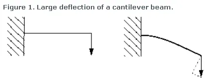
b) Material
Material nonlinearity is associated with the inelastic behavior of a component or system. Inelastic behavior may be characterized by a force-deformation (F-D) relationship, also known as a backbone curve, which measures strength against translational or rotational deformation.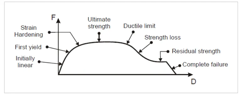
c) Contact
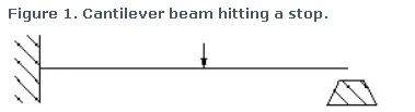
Boundary nonlinearity occurs if the boundary conditions change during the analysis. There is then a sudden change in the boundary condition at the tip of the beam, preventing any further vertical deflection, and so the response of the beam is no longer linear.
3) Evaluate the critical load for the column shown below following small displacement theory
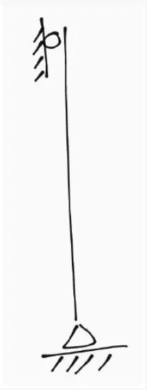
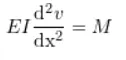
M is the internal bending moment at a given cross-section, v represents the lateral deflection of the column and the distance along the length of the column.EI is referred to as the flexural rigidity and is the product of Young’s modulus E and the second moment of area of the cross-section I.
Diffrenctial Equation establishment:-
Taking moments about point A yields:
Substituting M back into the differential equation of the deflection curve and rearranging slightly yields:
This is a linear, homogeneous, 2nd order differential equation with constant coefficients. It also happens to be an equation that models the deflected shape of our structure and contains P the axial load. Following the same approach as for the idealized structure discussed previously, if we solve this equation we can determine Pcr, the value of the applied load at which it is balanced by the column’s flexural bending resistance.
So we’re faced with trying to solve a differential equation. At this point, it’s helpful to be able to point to the general solution of this form of differential equation
Solving the differential equation:-
Boundary condition 1:
At (base of the column at pin support), (the lateral deflection must equal zero. Imposing these conditions on our general solution yields:
Therefore
As a result, our solution reduces to:
Boundary condition 2:
At (top of the column at pin support), (lateral deflection also zero). Again, imposing these boundary conditions yields,
So, either equals zero or equals zero. If equals zero, the equation is satisfied for any value of . This doesn’t really move us forward…we can think of this solution as the trivial solution. Of more interest is the case where:
Knowing what we know about functions, this equation can only be true, when,
We can dismiss the case where,
In this scenario, would need to equal zero (as all other terms have non-zero values by definition) and we know this is not the case. So for a pinned-pinned column, our solution is:
where...Finally, we can rearrange this equation to make the subject of the equation:
________________________________________________________________________________________________
4) Explain the concept of equilibrium with examples
a) Stable Equilibrium
A physical system made up of many parts is in mechanical equilibrium if the net force on each of its individual parts is zero. ... In terms of momentum, a system is in equilibrium if the momentum of its parts is all constant. In terms of velocity, the system is in equilibrium if velocity is constant.
A body is in stable equilibrium if it comes back to its normal position on slight displacement
Examples
(1) A ball in the valley between two hills. a small displacement of the ball toward either side will result in a force returning the ball to the original position. Thus the equilibrium is stable
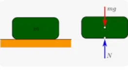
(2)A book lying on a horizontal surface is an example of stable equilibrium. If the book is lifted from one edge and then allowed to fall, it will come back to its original position
(3) A cone with a flat surface on the horizontal floor. If the clone is tilted slightly, it comes back to its normal position
b) Neutral Equilibrium
A body is said to be in neutral equilibrium if on being slightly displaced it remains in its new position, e.g a ball placed on a horizontal surface or a cone supported on its side on a horizontal surface.
If a ball is pushed slightly to roll, it will neither come back to its original nor it will roll forward rather it will remain at rest.
Examples:
(1) A ball on a flat surface. A small displacement will not have any impact on the ball.
c) Unstable Equilibrium
A state of equilibrium of a body (as a pendulum standing directly upward from its point of support) such that when the body is slightly displaced it departs further from the original position).
A body is in unstable equilibrium if it does come back to its normal position on slight displacement
Example
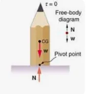
(1) pencil standing on its point or a stick in vertically standing position.
(2) thin rod standing vertically is slightly disturbed from its position it will not come back to its original position.
(3) Vertically standing cylinder
(4) A ball at the top of a rounded hill. A small displacement of the ball results in a force that moves the ball away from the equilibrium point so that equilibrium cannot be maintained.
______________________________________________________________________________________________________________
5) Develop a Matlab function to implement evaluation of critical load capacity of columns for different boundary conditions ( eg: Pin-Pin, Fixed-Fixed, Fixed- Free )
function [global_stiffness_matrix]=ComputeGlobalStiffnessMatrix()
%Get Element Info
[node_coord,element_no,element_node,length_element,element_geometry,element_dof]=GetElementInfo();
%Get Boundary Conditions Info
boundary_conditions=GetBoundary_Conditions();
%Get Nodal loads Info
node_loads = GetNodalLoads();


%Calculating Number Of Elements And Nodes
no_elements = size(element_no,1);
no_nodes = size(node_coord,1);

%Intializing Matrix with Zeros
global_stiffness_matrix= zeros(3*no_nodes,3*no_nodes);
displacement_matrix= zeros(3*no_nodes,1);
force_matrix = zeros(3*no_nodes,1);

%Boundary Conditions
all_dof= 1:3*no_nodes;
dof_specified =[]
for i=1:no_nodes
    n_dof=3*(boundary_conditions(i,1)-1)+boundary_conditions(i,2);
    dof_specified=[dof_specified n_dof];
    displacement_matrix(n_dof)=boundary_conditions(i,3);
end
free_dof=all_dof;
free_dof(dof_specified)=[]

%Compute Nodal Loads
for j =1:size(node_loads,1)
    force_matrix(3*(node_loads(j,1)-1)+node_loads(j,2))=node_loads(j,3);
end

%Global Stiffness Matrix
for k=1:no_elements
    ele_nodes=element_node(k,:);
    node_xy=node_coord(ele_nodes,:);
    A = element_geometry(k,1)*element_geometry(k,2);
    I=element_geometry(k,1)*element_geometry(k,2).^3/12;
    length=length_element(k);
    k_element=Frame_Stiffness_Matrix1(node_xy,A,I,length);
    eldofs=element_dof(k,:);
    global_stiffness_matrix(eldofs,eldofs)=global_stiffness_matrix(eldofs,eldofs)+k_element;

end
displacement_matrix(free_dof)=global_stiffness_matrix(free_dof,free_dof)\(force_matrix(free_dof)-global_stiffness_matrix(free_dof,dof_specified)*displacement_matrix(dof_specified));
force_matrix(dof_specified)=global_stiffness_matrix(dof_specified,:)*displacement_matrix;
disp('Displacement Vector');
disp(displacement_matrix);
disp('Force Vector');
disp(force_matrix);

end
Explanation of the above code:-
function [global_stiffness_matrix]=ComputeGlobalStiffnessMatrix()
%Get Element Info
[node_coord,element_no,element_node,length_element,element_geometry,element_dof]=GetElementInfo(); - taking data from the functions
%Get Boundary Conditions Info
boundary_conditions=GetBoundary_Conditions();
%Get Nodal loads Info
node_loads = GetNodalLoads();
%Calculating Number Of Elements And Nodes
no_elements = size(element_no,1);
no_nodes = size(node_coord,1);
%Intializing Matrix with Zeros
global_stiffness_matrix= zeros(3*no_nodes,3*no_nodes);
displacement_matrix= zeros(3*no_nodes,1);
force_matrix = zeros(3*no_nodes,1);
%Boundary Conditions
all_dof= 1:3*no_nodes;
dof_specified =[]
for i=1:no_nodes
n_dof=3*(boundary_conditions(i,1)-1)+boundary_conditions(i,2);
dof_specified=[dof_specified n_dof];
displacement_matrix(n_dof)=boundary_conditions(i,3);
end
free_dof=all_dof;
free_dof(dof_specified)=[]
%Compute Nodal Loads
for j =1:size(node_loads,1)
force_matrix(3*(node_loads(j,1)-1)+node_loads(j,2))=node_loads(j,3);
end
%Global Stiffness Matrix
for k=1:no_elements - for loop to iteration
ele_nodes=element_node(k,:); - assigning the elements nodes
node_xy=node_coord(ele_nodes,:); - assigning the coordinates for node x and node y
A = element_geometry(k,1)*element_geometry(k,2);
I=element_geometry(k,1)*element_geometry(k,2).^3/12;
length=length_element(k);
k_element=Frame_Stiffness_Matrix1(node_xy,A,I,length);
eldofs=element_dof(k,:);
global_stiffness_matrix(eldofs,eldofs)=global_stiffness_matrix(eldofs,eldofs)+k_element;
end
displacement_matrix(free_dof)=global_stiffness_matrix(free_dof,free_dof)\(force_matrix(free_dof)-global_stiffness_matrix(free_dof,dof_specified)*displacement_matrix(dof_specified));
force_matrix(dof_specified)=global_stiffness_matrix(dof_specified,:)*displacement_matrix;
disp('Displacement Vector');
disp(displacement_matrix);- display the dispacement amtrix
disp('Force Vector');- display the force vector name
disp(force_matrix);- display the force matrix
end
6) Develop an algorithm to implement matrix approach in the second-order elastic analysis
Input:-
Depict parameter for applied loading.
nodes, element, Moment of Intertia, Section Area, and Section length.
Processing:-
K(Stiffness matrix) is not constant
[[Ke]-[Kg]] =[Kt]
[Ke]+[Km]=Kt --- change with every iteration
1)Breaking load increment as second increment of force vector P
Ki[d`deltai`]=[dPi]
[dPi]=d`lamda`[P]
2)i=1 to n elements
{[Ke+Kg][d`deltai`]=[dPi]
3)Assemblies stiffness matrix] = d`'deltai` calculation from dPi`
References:
https://physicscatalyst.com/article/equilibrium-and-potential-energy/