Simulate an animation for the Simple Pendulum using MATLAB

Objective: -

Develop a program that solves the following ODE which represents the equation of motion of a simple pendulum with damping and simulate an animation for the simple pendulum.

Principle: -

The pendulum moves depend on Newton's second law. When this law is written down, we get a second order Ordinary Differential Equation that describes the position of the "ball" w.r.t time. A simple pendulum consists of a mass m hanging from a string of length L and fixed at a pivot point P. When displaced to an initial angle and released, the pendulum will swing back and forth with the periodic motion. By applying Newton's second law for rotational systems, the equation of motion for the pendulum may be obtained.

Solution procedure: -

ODE represents the equation of motion of a simple pendulum with damping

`(d^2θ)/(d^2t)+b/m*dθ/dt+g/L*sinθ=0`

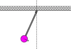
In the above equation,

g = gravity in m/s2,

L = length of the pendulum in m,

m = mass of the ball in kg,

b=damping coefficient.

we used,

L=1 metre,

m=1 kg,

b=0.05.

g=9.81 m/s2.

Simulation of the motion is done between 0-20 sec, for angular displacement=0,angular velocity=3 rad/sec at time t=0.

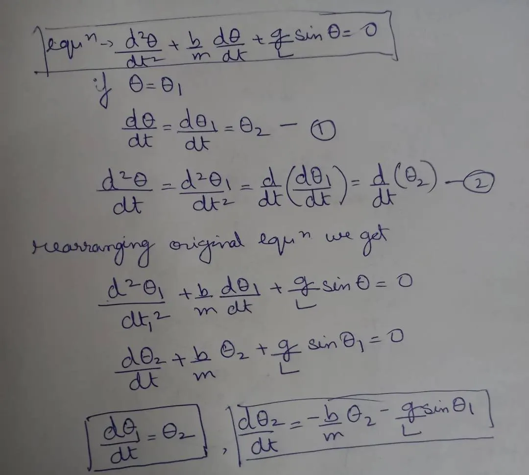
CODE for the function used: -

%Function to solve the ode
function [dtheta_dt] = pendulum_damped_ode(t,theta,b,g,l,m)
  
%Values intialized according to the equation
   theta1 = theta(1);
   theta2 = theta(2);
   dtheta1_dt = theta2;
   dtheta2_dt = -(b/m)*theta2 - (g/l)*sin(theta1);
   dtheta_dt =[dtheta1_dt; dtheta2_dt];
end

Explanation of the above CODE: -

• function [dtheta_dt] = pendulum_damped_ode(t,theta,b,g,l,m) - function is used to make the code easy to implement ,it is a group of statements that together perform a task
• theta1 = theta(1); - initializing as theta(1) according to the equation
• theta2 = theta(2); - initializing as theta(2) according to the equation
• dtheta1_dt = theta2; - initializing according to the equation
• dtheta2_dt = -(b/m)*theta2 - (g/l)*sin(theta1); - calculating dheta2/dt
• dtheta_dt =[dtheta1_dt; dtheta2_dt];
• end -to close the function
  

CODE for the animation of a simple pendulumand solving the equation for second order ode: -

clear all
close all
clc


g=9.81;
l=1;
m=1;
b=0.05;

%intial condition 
theta_0 = [0;3];

%time points
t_span =linspace(0,20,500);

%solve_ODE
[t, results] =ode45(@(t,theta) pendulum_damped_ode(t,theta,b,g,l,m),t_span,theta_0);

%plotting
subplot(5,4,[13,14,17,18]);
plot(t,results(:,1),'color','b')
hold on;
plot(t,results(:,2),'color','r');
hold off;
subplot(5,4,[15,16,19,20]);
plot(results(:,1),results(:,2));
xlabel('Position Radians');
ylabel('Angular Velocity');

ct=1;
for i = 1: length(results(:,1))
    x0=0;
    y0=0;
    x1=l*sin(results(i,1));
    y1=-l*cos(results(i,1));
    
    subplot(5,4,[1,2,3,4,5,6,7,8,9,10,11,12]);
    plot([-1 1],[0,0],'linewidth',4,'color','k');

    hold on
    line([x0 x1],[y0,y1],'linewidth',2,'color','b');
    hold on;
    
    %Plotting the bob using marker and facemaker
    plot(x1,y1,'-o','markers',20,'markerfacecolor','r');
    grid on;
    axis([-1.5 1.5 -1.5 0.5])
    pause(0.0003);

    hold off
     M(ct) = getframe(gcf);
    
    ct=ct+1;
    end
        
movie(M)
videofile= VideoWriter('pendulum_animation.avi','Uncompressed AVI')
open(videofile)
writeVideo(videofile,M)
close(videofile)

Explantion of the above code: -

• clear all - to clear all the workspace variables
• close all - to close all the output window
• clc - to clear the command window
• g=9.81; - initializing gravity as 9.81m/s
• l=1; -intializing length of the pendulum as 1 m
• m=1; - initializing mass of the ball as1 kg
• b=0.05; - initializing damping coefficient as 0.05
• %intial condition - comments to make the program user friendly
• theta_0 = [0;3]; - initializing the column of theta1 and theta2 as 0 and 3

time points

• t_span =linspace(0,20,500); - for simulation of the motion between 0-20 sec , linspace is used to generate 500 values between 0 and 20

solve_ODE

• [t, results] =ode45(@(t,theta) pendulum_damped_ode(t,theta,b,g,l,m),t_span,theta_0);

ODE45 is used to compare methods of orders four and five to estimate error and determine step size. ODE45 is so accurate that its default behavior is to use its interpolant to provide results at intermediate points.

The solver ode45 implements the Runge-Kutta(4,5) method. Such method is suited for solving ordinary differential equations by predictions.Runge–Kutta method is an effective and widely used method for solving the initial-value problems of differential equations. Runge–Kutta method can be used to construct high order accurate numerical method by functions' self without needing the high order derivatives of function

%plotting - comments are used to make the program user friendly

• subplot(5,4,[13,14,17,18]); - subplot divides the current figure into rectangular panes that are numbered row-wise
• plot(t,results(:,1),'color','b') - for the plotting
• hold on; - sets the hold state to on
• plot(t,results(:,2),'color','r'); - for the plotting
• hold off; - sets the hold state to off
• subplot(5,4,[15,16,19,20]);
• plot(results(:,1),results(:,2));
• xlabel('Position Radians'); - to label the x axis
• ylabel('Angular Velocity'); - to label y axis
• ct=1; - to initialize ct as 1
• for i = 1: length(results(:,1)) - for execution of the statements in loop
• x0=0; - initializing x0 as 0
• y0=0; - initializing y0 as 0
• x1=l*sin(results(i,1)); - initializing x1 coordinate value
• y1=-l*cos(results(i,1)); - initializing y1 coordinate value
• subplot(5,4,[1,2,3,4,5,6,7,8,9,10,11,12]);
• plot([-1 1],[0,0],'linewidth',4,'color','k');
• hold on;
• line([x0 x1],[y0,y1],'linewidth',2,'color','b');
• plot(x1,y1,'-o','markers',20,'markerfacecolor','r');- Plotting the bob using marker and facemaker
• grid on; - turn the grid on
• axis([-1.5 1.5 -1.5 0.5]) - initializing the axis limit range (-1.5 to 1.5) for x axis and (-1.5 to 0.5) for y axis
• pause(0.0003); - used to pause the video for 0.0003 sec to get asmotter plot and animation
• hold off
• M(ct) = getframe(gcf); - get frame for the plot
• ct=ct+1;
• end - used to close the loop
• movie(M) - plays the movie in matrix M once
• videofile= VideoWriter('pendulum_animation.avi','Uncompressed AVI') - additionally applies uncompressed avi properties tot his video to write data on avi file
• open(videofile) - used to open videofile for writing the video data
• writeVideo(videofile,M) - to write the video data to the file
• close(videofile) - used to close videofile for writing the video data

Output plot: -

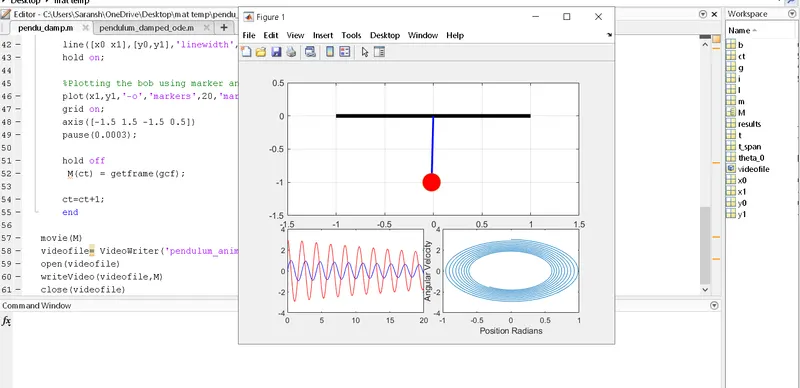
Youtube Link for the Animation: -

https://youtu.be/py6E176Xwws