Week 9.1: Turbo Charger Simulation Project

Note: Due to personal computer’s restricted ability, this report is prepared based on a simulation with coarse mesh of size 0.008m instead of finer mesh size.

Aim: To carry out a simulation of air flow inside a Turbocharge using Converge 3.0 CFD program and then post-process the results on Paraview.

Introduction: We need to observe the parameters of Air as a medium flowing inside a Turbocharger. In this simulation we can examine the rotation of the turbine wheel due to difference in the inlet and outlet pressure. The pressure ratio creates the necessary momentum for the wheel due to which it starts to rotate. In automotive applications this wheel is then connected to a compressor shaft. The compressor is basically used to increase the volumetric efficiency to bring in more air into the engine. The turbocharger selection will then be based upon the amount of air to be brought inside the engine.

The simulation time and the speed of the turbine wheel are decided based on a compressor map. The compressor map is a graph which describes the performance characteristics of a compressor such as turbocharger speed, mass flow rate, pressure ratio, efficiency etc. Once the amount of air to be forced inside is decided for the compressor, this map based on the efficiency and pressure ratio will help in selecting the rotational speed for a turbrocharger. The rotational speed of the wheel helps in deciding the simulation time required for the turbine wheel to reach necessary rotational speed.

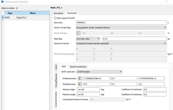
Traditionally a turbocharger is run with the help of exhaust gases after combustion from the engine. This particular simulation also makes use of Fluid-Structure Interaction (FSI). Since the incoming gases rotates the turbine wheel and depending upon the enthalpy of the air the speed is going to change. So, we use this model to simulate the interaction of the fluid (i.e. Hot Air) with the solid (i.e. Turbine Wheel).

The other parameters to be observed are change in the velocity, pressure, mass flow rate through-out the flow and total cell count.

We used three different pressure ratios to run the simulation, which are as below:

1. Case 1: Pressure Ratio = 2
2. Case 2: Pressure Ratio = 2.5
3. Case 2: Pressure Ratio = 3

Simulation End Time Calculation:

Based on the compressor map inference can be drawn that the turbine rotates at approx. 1,00,000 RPM i.e. 1666.67 RPS for a pressure ratio of 2.5 and 77% efficiency.

Time taken for 1 rotation = 1 / 1666.67 = 0.0006 seconds (approx.)

So, End Time considering 10 rotations = 0.0006 x 10 = 0.006 seconds.

Geometry:

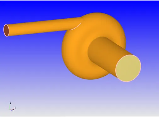
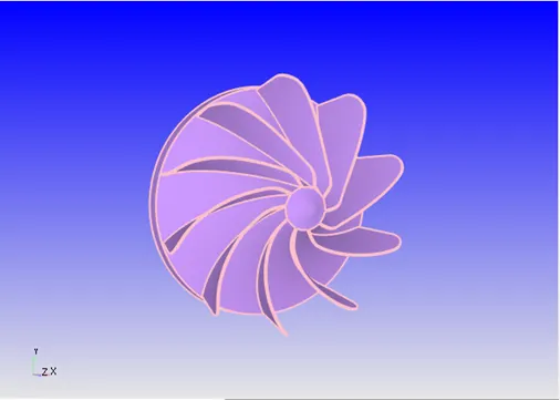
- In the Converge Studio first we import the ‘STL’ file of the geometry.

- Then, we carry out a ‘Diagnosis’ on the shape created to check for any errors. If there is no error then the geometry is correct.

- Then we move to case set up.

Case Set up Procedure:

- Application Type: Time-based

- Material: Predefined Mixture = Air

- Select Gas Simulation & Reaction Mechanism.

- Reaction Mechanism: Gas Species O₂ & N₂ are the available species in the air.

- Simulation Parameters:

- Run Parameter: Transient Solver used to perform with Full Hydrodynamic mode.

- Simulation Time Parameter:

- End Time = 0.006 second.

- Maximum Time Step = 1 second

- Maximum Convection CFL limit = 1

- Solver Parameters:

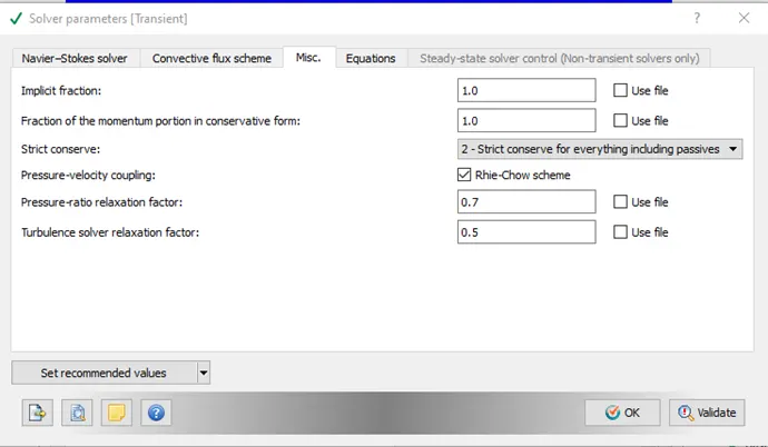
- Navier-Stokes Solver Type = ‘Density based’ selected.

- Misc. Setting:

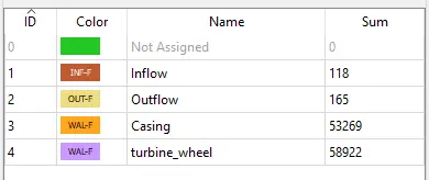
- Boundary Conditions:

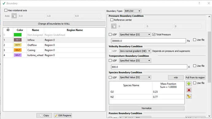
- Inflow: Inlet Pressure – Case-1 = 200000 Pa;

Case-2 = 250000 Pa;

Case-3 = 300000 Pa.

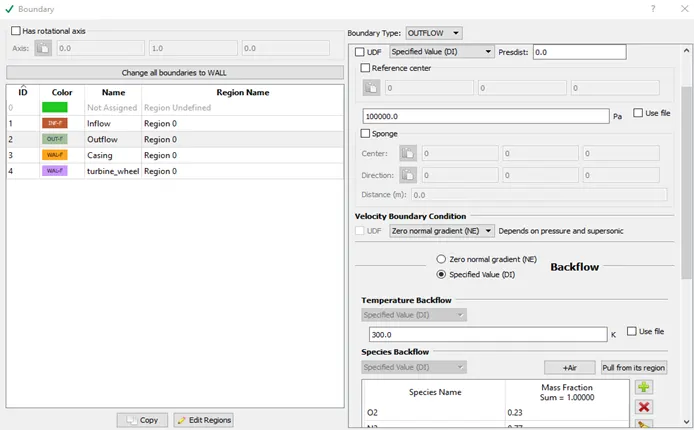
- Outflow: Outlet Pressure = 100000 Pa

- Inflow Boundary Condition:

Case-1- Inlet Pressure = 200000 Pa; Temp. = 800 K.

Case-2- Inlet Pressure = 250000 Pa; Temp. = 800 K.

Case-3- Inlet Pressure = 300000 Pa; Temp. = 800 K.

- Outflow Boundary Condition: Pressure = 100000 Pa; Temp. = 300 K.

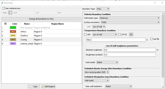
- Casing Boundary condition: Temp. = 450 K.

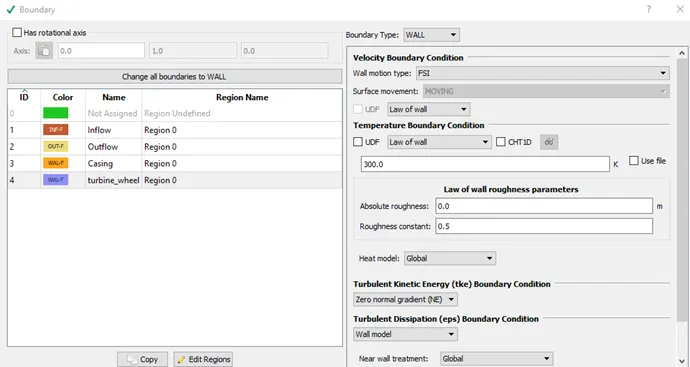
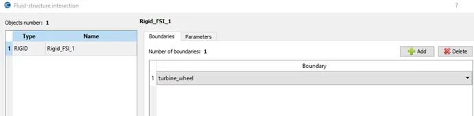
- Turbine-Wheel Boundary Condition: Wall with “FSI”.

- Initial Conditions & Events:

- Regions: All boundaries defined to ‘Region 0’.

Initial Pressure = set to 101325 Pa; Temp. = 500 K.

- Species Mass Fraction: O₂ = 0.23; N₂ = 0.77

- Physical Models:

- Turbulence Modelling= set to RANS [RNG K-Ɛ]

- Fluid-Structure Interaction (FSI) selected:

- Grid Control:

Base Grid Size: dx = dy = dz = 0.008m

- Post Processing:

- Post variables Selection:

- Typical Variables/Geometry: Select desired variables such as Density, Velocity, pressure, temperature.

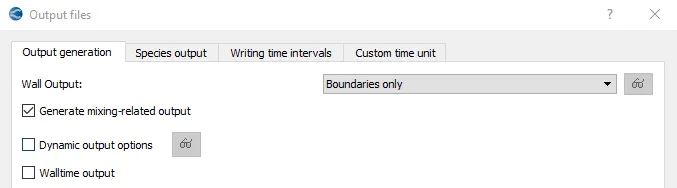
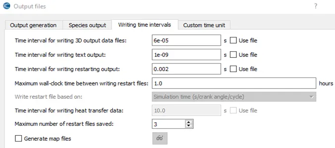
- Output Files:

Case setup is complete with this.

- Export case setup: The case setup files are then ‘Exported’ to the destination folders to save the details.

- The destination folders should consist of following files in order to run the simulation and then post process the result on Paraview. The files are:

(i) converge.exe (name changed for the ease of run command on cygwin)

(ii) mpiexec.exe (name changed for the ease of run command on cygwin)

(iii) post_convert.exe (under output folder)

- Open Cygwin: Now the simulation is run using Cygwin. We navigate to the desired folder where the setup files were exported.

- Command to Run Simulation: The command to run simulation through Cygwin for Converge Studio 3.0 version is as below:

“ mpiexec.exe –n 2 converge.exe restricted “

• The simulation starts running, due to which output files are generated under a separate output folder.
• These output files are then post processed to convert the data in a format suitable for Paraview.

• Inline Plot: In the Converge Studio program, we can use Inline Plotting option to plot the curves during simulation run. We can observe the change in the plots and see the position of the simulation at the end of the time.

• Post Convert in Converge: To post process, we use file type as ‘Paraview VTK in-line binary format’. Now the files are post processed with a case name ‘test’.

• This generates ‘test.vtm’ group files which are generally used in Paraview to observe the results.

• Paraview: Open Paraview to check for the results.

Observations for All Cases:

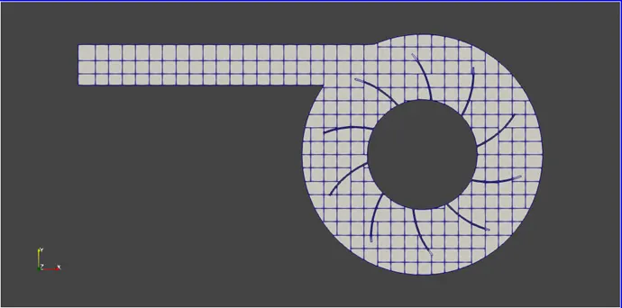
Mesh Formation:

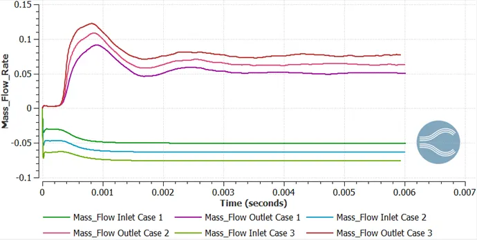
Mass Flow Rate Plot:

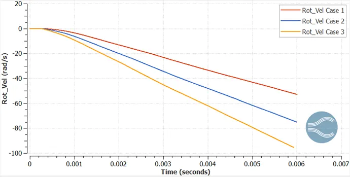
Rotation Velocity Plot:

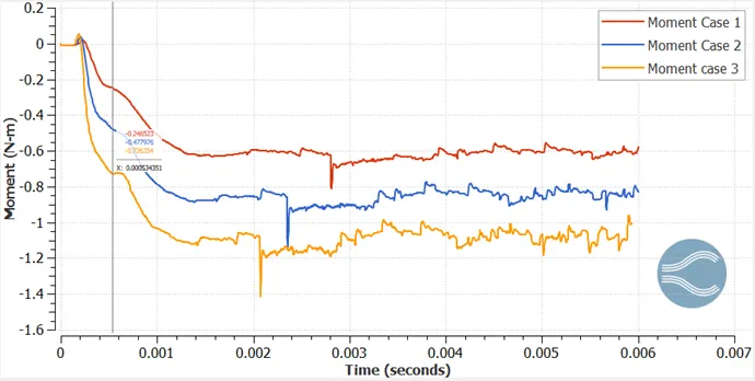
Momentum Plot:

Total Cell Count:

Average Velocity Plot:

Pressure-Velocity Animation:

https://youtu.be/qGrMdiWbyak

Temperature-Wheel Animation:

https://youtu.be/jSIBHmPIV8w

Results:

After running the simulation, the results can be observed as below:

1. The Rotation Velocity increases with the increase in the pressure ratio which is 52 rad/s, 75 rad/s, 95 rad/s respectively for case 1, 2, & 3.
2. We can also infer from the Rotation velocity plot that the turbine wheel is still in motion even after the end time and it has not reached it necessary speed. So the simulation is needed to be run for the longer duration in order to capture the effects when the wheel reaches it maximum speed.
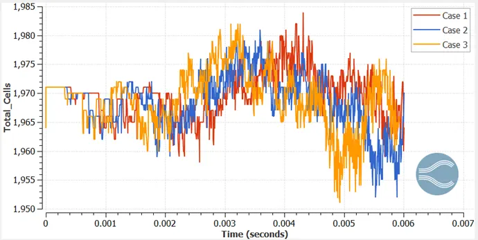
3. The cell count plot shows fluctuation but this is due to rotation of the wheel which intermittently cuts the cells. At the start the cell count is minimal; this is because the impeller is yet to overcome its inertia and then starts to rotate slowly. Thus the cell count fluctuations are more towards the end.
4. This simulation uses a very important concept of Fluid-Structure Interaction (FSI) which helps in determining the effects of interaction of fluid with the solid surface.
5. The mass flow rate plot indicates that the flow has converged within 0.006 seconds.
6. The momentum plot shows that the average torque to rotate the turbine wheel is around 0.6 Nm, 0.85 Nm, 1 Nm respectively for case 1, 2, & 3.
7. So, this simulation time of 0.006 seconds is enough to see whether the the mass flow rate is converged or whether the necessary torque is attained to rotate the turbine. If we want to see when the turbine reaches its maximum speed for the given pressure ratios then the simulation time needs to be longer.
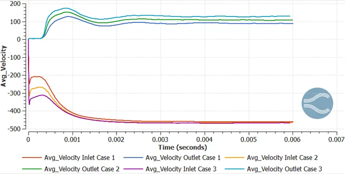
8. The Average velocity plot shows that the velocity at the intlet in all the three cases is at a value of 465 m/s (max.) which gives an initial momentum and the wheel slowly starts to rotate. At the end of simulation time the outlet velocity seems to have converged with the values of 89 m/s, 107 m/s & 129 m/s respectively.
9. The pressure animation shows that with difference in pressure the wheel starts to rotate. The flow also hits the back of the blade of turbine which creates some resistance to the rotation.

Speed of Impeller:

Case	Pressure Ratio	Rotational Velocity (Rad/s)	Speed of Impeller (RPM)
1	2	52	497
2	2.5	75	720
3	3	95	907

Calculation of Time for Maximum Speed of Turbine Wheel:

In this simulation, with a pressure ratio of 2.5, the rotational velocity obtained is 75 Rad/s or 720 RPM.

The turbochargers are usually run at a speed of approx. 1,50,000 RPM.

For 720 RPM - - - - 0.006 seconds.

So, for 1,50,000 RPM - - - - ( 0.006 x 150000 ) / 720 = 1.25 seconds.

Therefore, if the simulation is run for 1.25 seconds, then the turbine wheel will reach it maximum speed.

Conclusion:

We can conclude from the simulation using Converge CFD program that:

• Simulation was run for three different pressure ratios successfully.
• The FSI method was used and the results obtained can be used to work out the stress on the solid structure.
• The run time needs to be longer to capture the maximum speed of the turbine wheel and then obtaining the effects on the material due to
• The change in the parameters for a flow can be observed from the various animations, plots, contours and profiles.