Week 3: Flow over a backward facing step
BACKWARD FACING STEP SIMULATION:
Aim: To carry out a simulation of air flow over a Backward Facing Step using Converge 3.0 CFD program and then post-process the results on Paraview.
Introduction: We need to observe the parameters of Air as a medium flowing inside a Backward Facing Step of specific sizes. In this simulation we can examine the separation of flow from the boundary and backward flow of air near the expanded area. The parameters to be observed are change in the velocity, pressure, mass flow rate through-out the flow.
We used three different Base grid sizes for the channel, which are as below:
- Case 1: Base Grid (in m): dx = dy = dz = 2e-3
- Case 2: Base Grid (in m): dx = dy = dz = 1.5e-3
- Case 2: Base Grid (in m): dx = dy = dz = 1e-3
Creating Geometry:
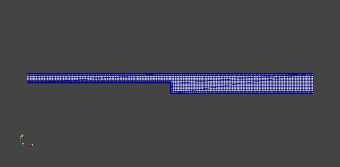
- In the Converge Studio first we create the geometry of a Backward facing Step’ as shown below:
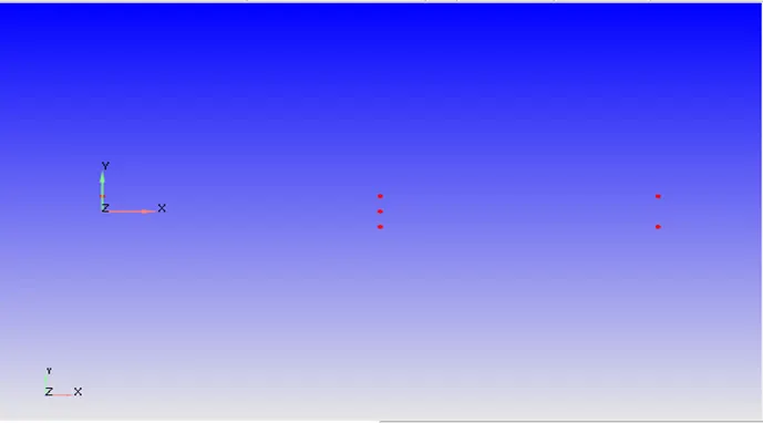
(i) Vertices were drawn first on the proper distances across X & Y directions.
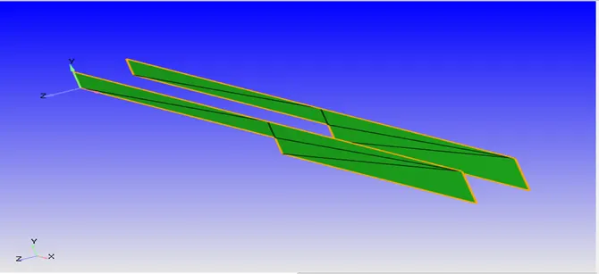
(ii) Triangles created to form one face of the geometry. The face is copied at a distance of 0.02m on the negative Z axis. Thus a second face of the geometry is formed.
(iii) These two faces were then joined by ‘Loft Edges’ function. Thus the geometry formation is complete.
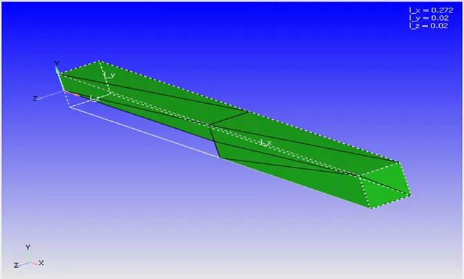
- Then, we carry out a ‘Diagnosis’ on the shape created to check for any errors. If there is no error then the geometry is correct.
- Then, check for the vector ‘Normal’, initially the normal points out of the shape, which are then transformed to point inward. Since the flow is inside the channel, so the correct position for the normal should be pointing inward.
- Now the correct geometry is created, so we move to case set up.
Case Set up Procedure:
- Application Type: Time-based
- Material: Predefined Mixture = Air
- Select Gas Simulation & Reaction Mechanism.
- Reaction Mechanism: Gas Species O2 & N2 are the available species in the air.
- Simulation Parameters:
- Run Parameter: Steady State Solver used. Steady State Monitor is Turned On.
- Steady State Monitor: Monitor variables added such as Avg. Velocity, Total Pressure. These variables are monitored at the ‘outlet’.
- Simulation Time Parameter:
- End Time = 15000 cycles.
- Maximum Time Step: Case-1 = 1 s; Case-2 = 2 s; Case-3 = 1 s;
- Maximum Convection CFL limit = 1
- Solver Parameters:
- Navier-Stokes Solver Type = ‘Density based’ selected.
- Equations Tab: Pressure Pre-conditioner set to ‘None’.
- Steady State Solver control: Maximum Convection CFL limit (final stage) = 0.5.
- Boundary Conditions:
- Inflow: Inlet Pressure – Case-1 = 110325 Pa; Case-2 = 110325 Pa; Case-3 = 111325 Pa
- Outflow: Outlet Pressure = 100000 Pa
- Top / Bottom Walls = ‘Stationary’ Walls with ‘Law of the Wall’ condition.
- Front / Back Walls = set to 2D.
- Initial Conditions & Events:
- Regions: Initial Pressure = set to 101325 Pa. All boundaries defined to ‘Region 0’
- Species Mass Fraction: O2 = 0.23 ; N2 = 0.77
- Physical Models:
- Turbulence Modelling= set to RANS [RNG K-Ɛ]
- Grid Control:
Base Grid with Fixed Embedding:
- Case 1: Base Grid (in m): dx = dy = dz = 2.0e-3.
- Case 2: Base Grid (in m): dx = dy = dz = 1.5e-3.
- Case 3: Base Grid (in m): dx = dy = dz = 1.0e-3.
- Post Processing:
- Post variables Selection:
- Typical Variables/Geometry: Select desired variables such as Density, Velocity, pressure, temperature.
- Output Files:
- Time Interval for writing 3D output data files = 1000 cycles
- Time interval for writing restarting output = 1000 cycles
- Maximum number of restart files saved = 3.
Case setup is complete with this.
- Export case setup: The case setup files are then ‘Exported’ to the destination folders to save the details.
- The destination folders should consist of following files in order to run the simulation and then post process the result on Paraview. The files are:
(i) converge.exe (name changed for the ease of run command on cygwin)
(ii) mpiexec.exe (name changed for the ease of run command on cygwin)
(iii) post_convert.exe (under output folder)
- Open Cygwin: Now the simulation is run using Cygwin. We navigate to the desired folder where the setup files were exported.
- Command to Run Simulation: The command to run simulation through Cygwin for Converge Studio 3.0 version is as below:
“ mpiexec.exe –n 2 converge.exe restricted “
- The simulation starts running, due to which output files are generated under a separate output folder.
- These output files are then post processed to convert the data in a format suitable for Paraview.
- Inline Plot: In the Converge Studio program, we can use Inline Plotting option to plot the curves during simulation run. We can observe the change in the plots and see the simulation reach the steady state condition at the end of the plot.
- Post Convert in Converge: To post process, we use file type as ‘Paraview VTK in-line binary format’. Now the files are post processed with a case name ‘test’.
- This generates ‘test.vtm’ group files which are generally used in Paraview to observe the results.
- Paraview: Open Paraview to check for the results.
- Observations for Case 1:
Base Grid (in m): dx = dy = dz = 2.0e-3.
Fixed Embedding: Scale = 2; Layer = 1.
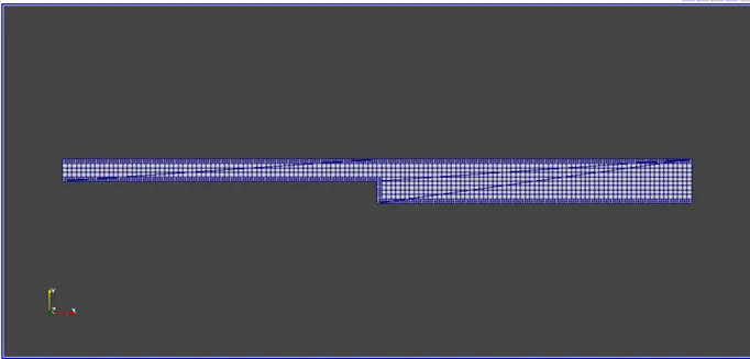
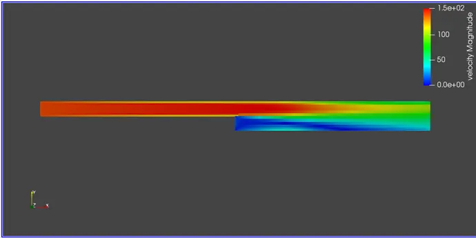
Velocity Contour:
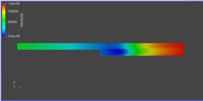
Pressure Contour:
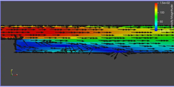
Flow Separation Contour:
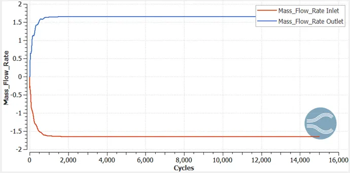
Mass Flow Rate Plot:
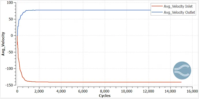
Velocity Plot:
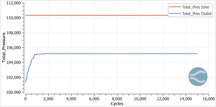
Total Pressure Plot:
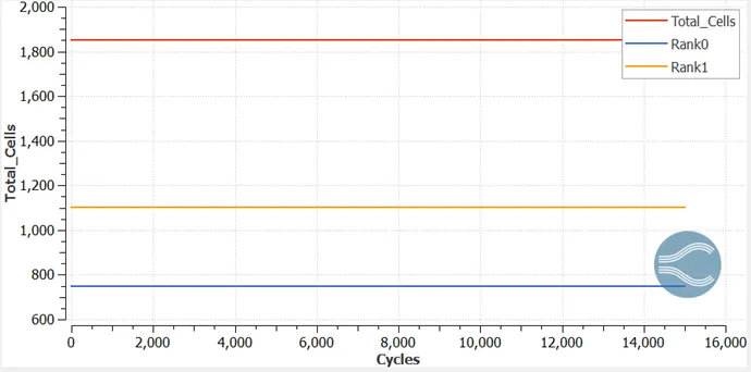
Total Cell Count:
Velocity Animation:
Pressure Animation:
(B) Observations for Case 2:
- Base Grid (in m): dx = dy = dz = 1.5e-3.
- Fixed Embedding: Scale = 2; Layer = 2.
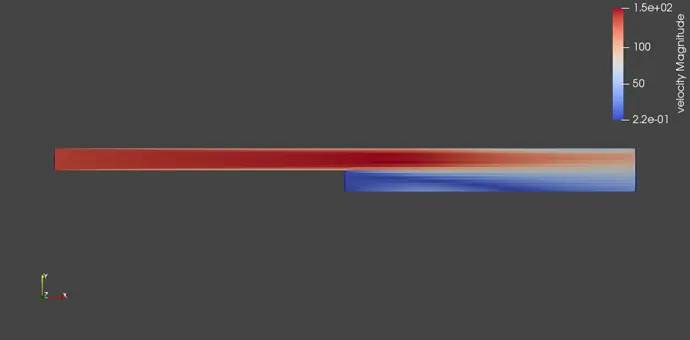
Velocity Contour:
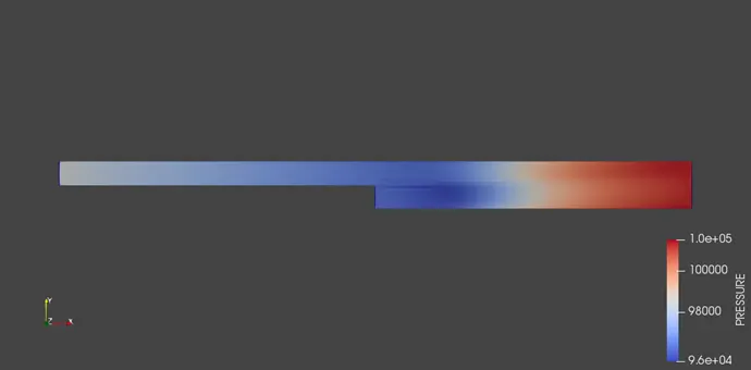
Pressure Contour:
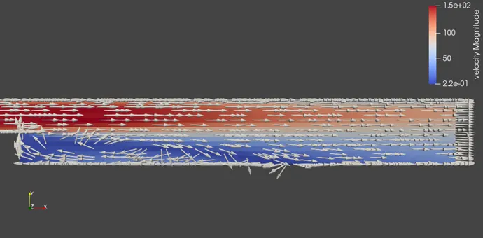
Flow Separation Contour:
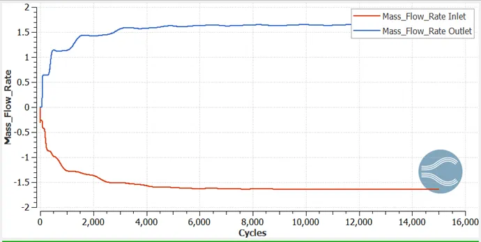
Mass Flow Rate Plot:
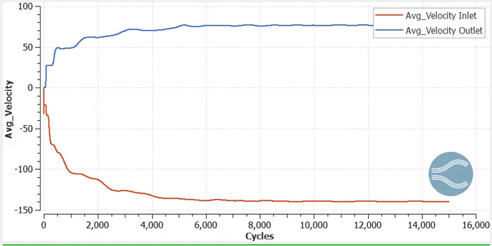
Velocity Plot:
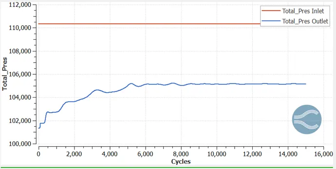
Total Pressure Plot:
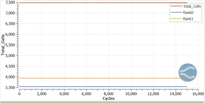
Total Cell Count:
Velocity Animation:
Pressure Animation:
(C) Observation for Case 3:
- Base Grid (in m): dx = dy = dz = 1.0e-3.
- Fixed Embedding: Scale = 2; Layer = 1
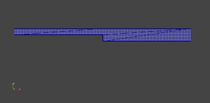
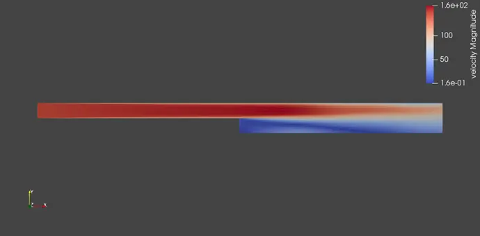
Velocity Contour:
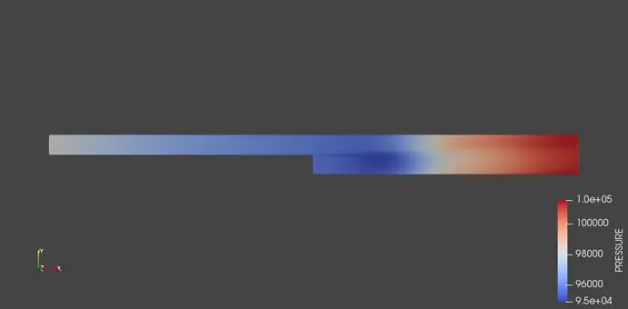
Pressure Contour:
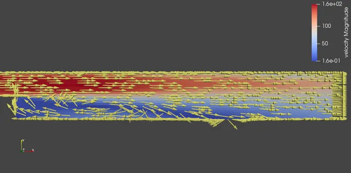
Flow Separation Contour:
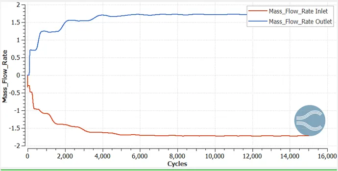
Mass Flow Rate Plot:
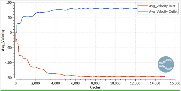
Velocity Plot:
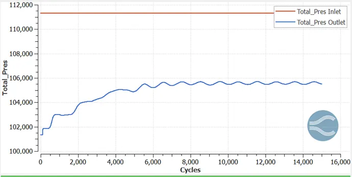
Total Pressure Plot:
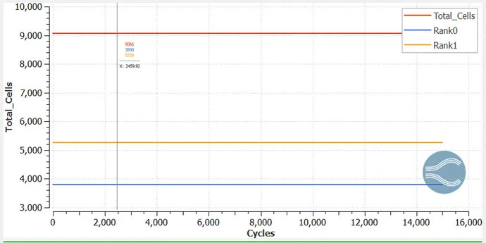
Total Cell Count Plot:
Velocity Animation:
Pressure Animation:
Results:
- Based on three different Base Mesh Sizes i.e. 2e-3m, 1.5e-3m & 1.2 e-3m, one can observe that with the finer mesh sizes the accuracy of results improves.
- The increase in Fixed Embedding scale and layers help in capturing the refinement of the simulation contour which is visible in case 2 & 3.
- The improvement in capturing the accuracy of the parameters can be attributed to the increase in the Total Cell Count i.e. 1851, 7478 & 9066 for three different cases respectively.
- The duration for simulation increases with increase in the cell count i.e. 422s, 1094s, 1435s respectively.
- The flow takes place due to difference in pressure at inlet and outlet.
- The change in the velocity can be observed with finer details due to refinement of mesh sizes.
- The Glyph vectors plot shows the flow separation and recirculation near the step prominently.
- The mass flow rate at the inlet and outlet for all three cases is conserved through-out the flow.
- After initial turbulence a steady state is reached in the end of the cycle, which can be visualized from the various plots.
Explanation of Results:
With the results obtained, we can infer that-
- The flow separation near the boundaries occurs due to rise of pressure at the outlet, which in turn causes reversal of flow. The total pressure at the outlet increases to 105500 Pa which can be seen in the Pressure plot.
- Turbulence in the flow is created and a turbulent region is visible near the step. Near the region of more cross-sectional area the flow starts to recirculate. This causes the increase in velocity at the step.
- The Velocity is gradually increasing near the top wall but a considerable drop in is observed near the bottom walls as the flow moves towards outlet. Due to expansion in area the velocity reduces from approx. 146 m/s to 80 m/s. This change in velocity is clearly seen in the velocity plots.
- So, this simulation helps in study of effects of flow reversal and turbulence at the backward facing step of any material.
Conclusion:
We can conclude from the simulation using Converge CFD program, that with finer mesh sizes the results obtained become prominent and accurate. The change in the parameters for a flow can be observed from the various animations, plots, contours and profiles and understand how the results reach steady state.