Week 6: Conjugate Heat Transfer Simulation

CONJUGATE HEAT TRANSFER FLOW SIMULATION:

Aim: To carry out a simulation of air flow through a pipe and perform a Conjugate Heat Transfer flow simulation using Converge 3.0 CFD program and then post-process the results on Paraview.

Introduction: Conjugate heat transfer occurs when heat transfer occurs simultaneously within and between the solid and fluid regions. The heat transfer between the fluid is through convection and between the solid through conduction.

Converge solves the fluid heat transfer using energy equation (Navier-Stokes Equation). Solid heat transfer is solved with the help of Three Dimensional Transient Heat Conduction equation (Energy Equation).

A process of Time Control i.e. Super Cycling is used in Converge to perform the simulation. The heat transfer rate in solids and fluids is different. The solids usually take more time to heat more than a fluid. So, when super cycling is used, the fluid simulation is performed with Transient method and solid simulation is performed with Steady-state method. The converge freezes the fluid solver until the solid side parameters reach the same time scale. The temperature distribution process becomes accurate in both the regions by super cycling.

Finally, we need to observe the parameters of Air as a medium flowing inside a pipe of specific sizes. The parameters to be observed are change in the velocity, temperature & Y⁺, Total cell count.

Formula to Calculate Velocity:

Re = (rho*V*D)/(Dynamic viscosity)

Where-

Reynolds Number (Re) = 7000

Air Density (Rho) @ 300 K = 1.165 Kg/m³

Inner Diameter of Pipe (D) = 0.04 m

Dynamic Viscosity @ 300 K = 1.85e-5 Kg/m.s

Velocity = 2.78 m/s (Calculated)

We used three different Base grid sizes for the channel, which are as below:

1. Case 1: Base Grid (in m): dx = dy = dz = 0.004
2. Case 2: Base Grid (in m): dx = dy = dz = 0.0035
3. Case 2: Base Grid (in m): dx = dy = dz = 0.0025

Creating Geometry:

- In the Converge Studio first we create the geometry of a Pipe as shown below:

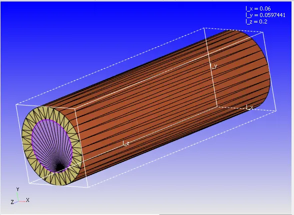
- Then, we carry out a ‘Diagnosis’ on the shape created to check for any errors. If there is no error then the geometry is correct.

- Then, check for the vector ‘Normal’, initially the normal points out of the shape, which are then transformed to point inward. Since the flow is inside the pipe, so the correct position for the normal should be pointing inward.

- Now the correct geometry is created, so we move to case set up.

Case Set up Procedure:

- Application Type: Time-based

- Material: Predefined Mixture = Air

- Select Gas Simulation, Solid simulation, Species.

- Gas Simulation: Redlich-Kwong

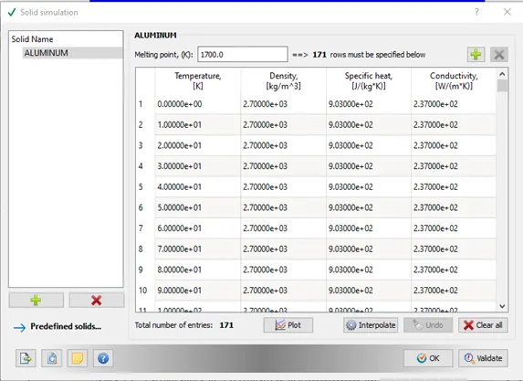
- Solid Simulation:

- Global Transport:

• Turbulent Prandtl Number = 0.9
• Turbulent Schmidt Number = 0.78

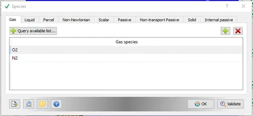
- Species: Gas Selection as below:

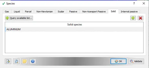
- Species: Solid Selection as below:

- Simulation Parameters:

- Run Parameter: Transient Simulation; Full hydrodynamic mode.

- Simulation Time Parameter:

- End Time = 0.5 s.

- Initial Time Step = 1e-7 s; - Minimum Time Step = 1e-7s.

- Maximum Time Step: 1 s;

- Maximum Convection CFL limit = 1

- Solver Parameters:

- Navier-Stokes Solver Type = ‘Density based’ selected.

- Misc.: Strict Conserve = 2-strict conserve for everything including passives.

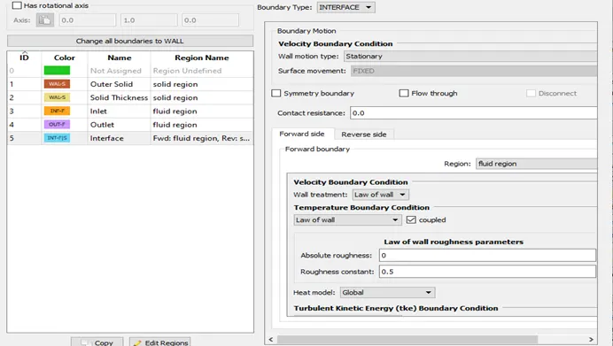
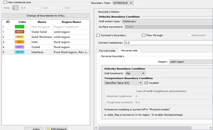
- Boundary Conditions:

- Outer Solid Boundary Condition:

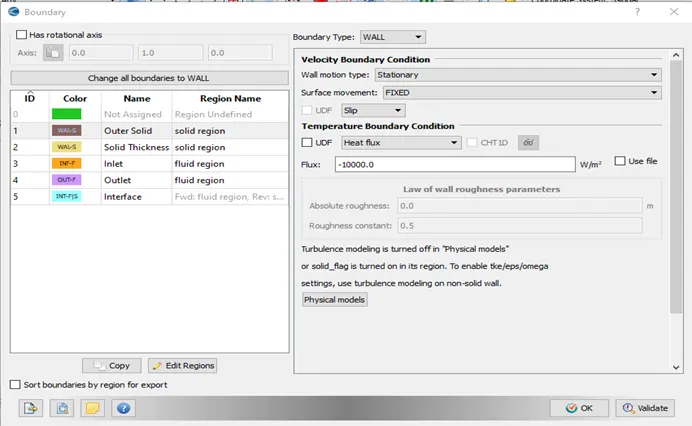
- Solid Thickness Boundary Condition:

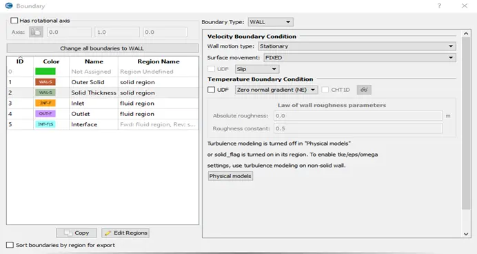
- Inlet Boundary Condition:

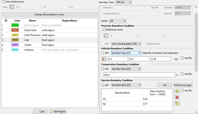
- Outlet Boundary Condition:

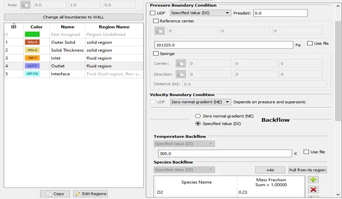
- Interface Conditions: Forward side conditions:

- Interface: Reverse Side Conditions:

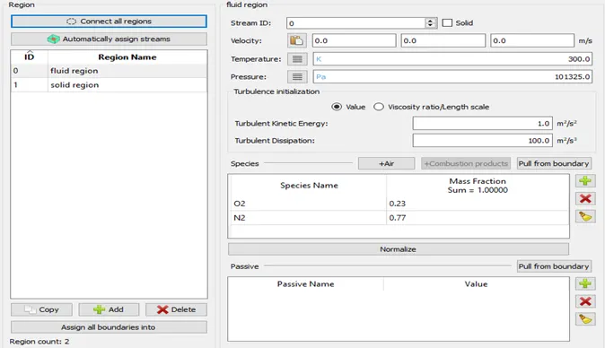
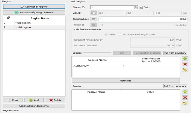
- Initial Conditions & Events: Regions & Initializations:

- Region- Fluid:

- Region- Solid:

- Physical Models:

- Turbulence Modelling= set to RANS [RNG K-Ɛ]

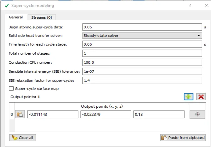
- Super Cycling:

- Grid Control:

Base Grid:

1. Case 1: Base Grid (in m): dx = dy = dz = 0.004.
2. Case 2: Base Grid (in m): dx = dy = dz = 0.0035.
3. Case 3: Base Grid (in m): dx = dy = dz = 0.0025.

- Post Processing:

- Post variables Selection:

- Typical Variables/Geometry: Select desired variables such as Density, Velocity, pressure, temperature.

- Combustion/Turbulence: Select Y⁺

- Output Files:

- Time Interval for writing 3D output data files = 0.01 s.

- Time interval for writing restarting output = 0.01 s.

- Maximum number of restart files saved = 3.

Case setup is complete with this.

- Export case setup: The case setup files are then ‘Exported’ to the destination folders to save the details.

- The destination folders should consist of following files in order to run the simulation and then post process the result on Paraview. The files are:

(i) converge.exe (name changed for the ease of run command on cygwin)

(ii) mpiexec.exe (name changed for the ease of run command on cygwin)

(iii) post_convert.exe (under output folder)

- Open Cygwin: Now the simulation is run using Cygwin. We navigate to the desired folder where the setup files were exported.

- Command to Run Simulation: The command to run simulation through Cygwin for Converge Studio 3.0 version is as below:

“ mpiexec.exe –n 2 converge.exe restricted “

• The simulation starts running, due to which output files are generated under a separate output folder.
• These output files are then post processed to convert the data in a format suitable for Paraview.
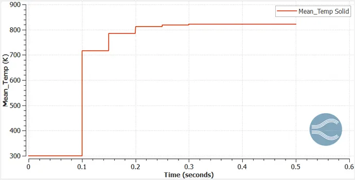
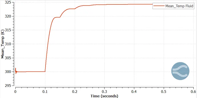
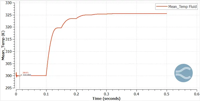
• Inline Plot: In the Converge Studio program, we can use Inline Plotting option to plot the curves during simulation run. We can observe the change in the plots and see the simulation reach the steady state condition at the end of the plot.
• Post Convert in Converge: To post process, we use file type as ‘Paraview VTK in-line binary format’. Now the files are post processed with a case name ‘test’.
• This generates ‘test.vtm’ group files which are generally used in Paraview to observe the results.
• Paraview: Open Paraview to check for the results.

(A) Observations for Case 1:

Base Grid (in m): dx = dy = dz = 0.004.

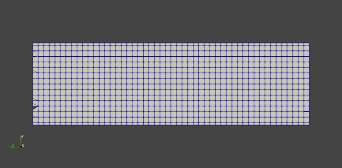
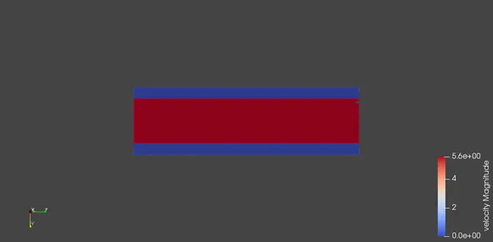
Velocity Contour:

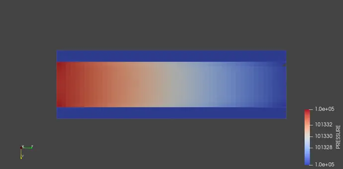
Pressure Contour:

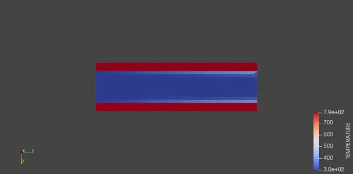
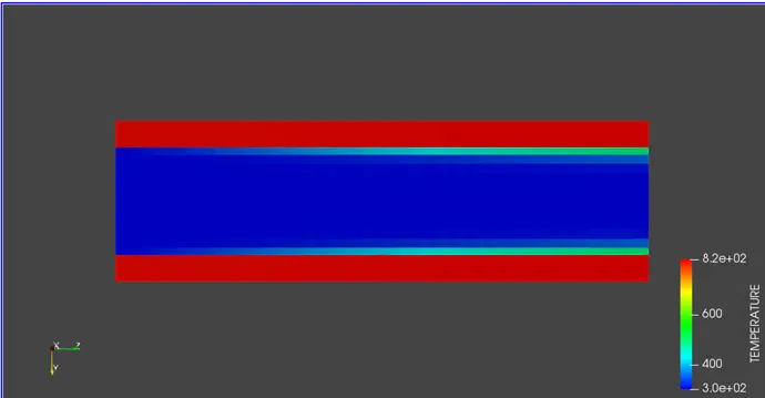
Temperature Contour:

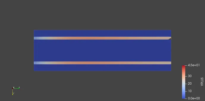
Y⁺ Contour:

Solid Mean Temperature Plot:

Fluid Mean Temperature Plot:

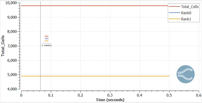
Total Cell Count:

Velocity Animation: https://youtu.be/RRgh4xJVk_8

Temprature Animation: https://youtu.be/Ps436QqRDF8

(B) Observations for Case 2:

- Base Grid (in m): dx = dy = dz = 0.0035.

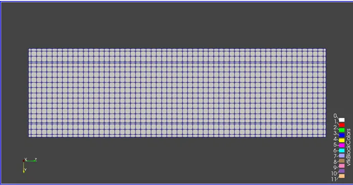
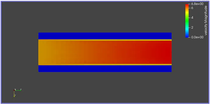
Velocity Contour:

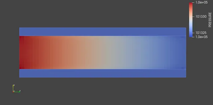
Pressure Contour:

Temperature Contour:

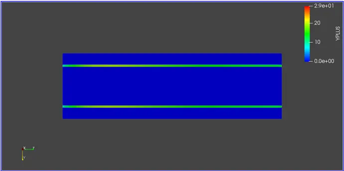
Y⁺ Contour:

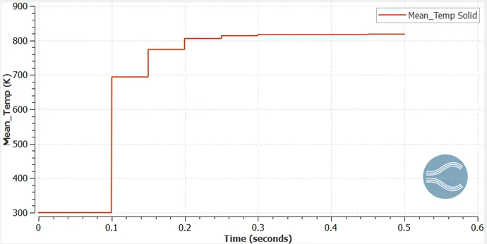
Solid Mean Temperature Plot:

Fluid Mean Temperature Plot:

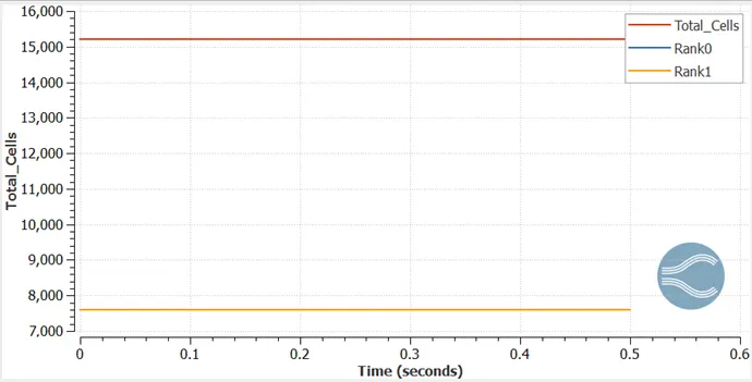
Total Cell Count:

Velocity Animation: https://youtu.be/PpGPsj7FQ7U

Temperature Animation: https://youtu.be/hasRfhkLeRE

(C) Observation for Case 3:

- Base Grid (in m): dx = dy = dz = 0.0025.

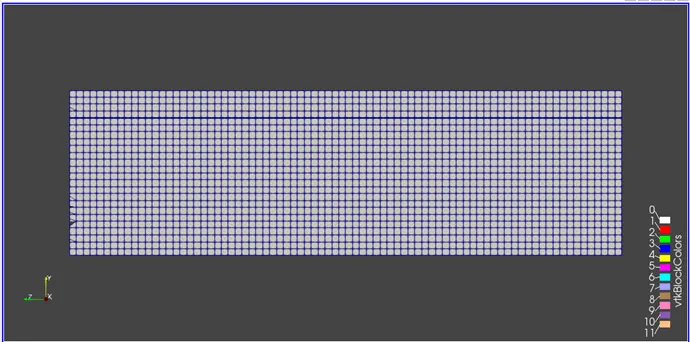
Velocity Contour:

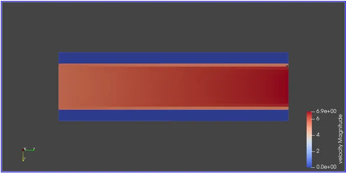
Pressure Contour:

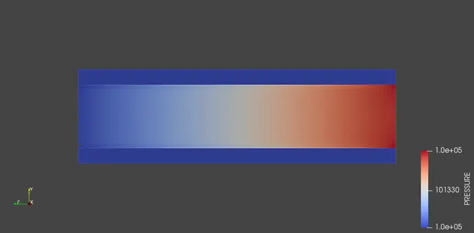
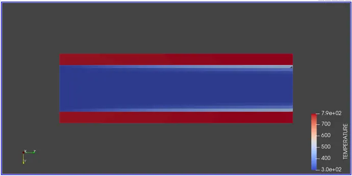
Temperature Contour:

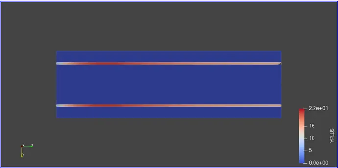
Y⁺ Contour:

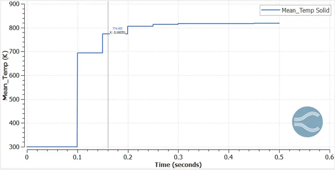
Solid Mean Temperature Plot:

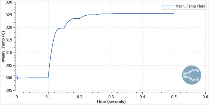
Fluid Mean Temperature Plot:

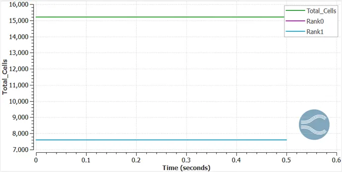
Total Cell Count:

Velocity Animation: https://youtu.be/Vim48qCL9KQ

Temperature Animation: https://youtu.be/AuYGz9AbB7A

Effects of Super-Cycling Intervals: Base Mesh = 0.004m used for the below cases -

Super Cycle Stage Interval = 0.05 ; Simulation Time = 1430 s

Super Cycle Stage Interval = 0.03 ; Simulation Time = 1173 s

Super Cycle Stage Interval = 0.02 ; Simulation Time = 943 s

Super Cycle Stage Interval = 0.01 ; Simulation Time = 1198 s

Results:

• Based on three different Base Mesh Sizes i.e. 0.004m, 0.0035m & 0.0025m, grid dependence test is carried out to observe the conditions of various parameters.
• The solid region temperatures are captured more prominently with decrease in mesh sizes.
• With reduction in Super cycling time interval the simulation time usually decreases.
• The Y⁺ values tend to decrease with finer mesh sizes.

Conclusion:

We can conclude from the simulation using Converge CFD program, that with finer mesh sizes the results obtained become prominent and accurate. The change in the parameters for a flow can be observed from the various animations, plots, contours and profiles and understand how the results reach steady state.