Week 8 - Simulation of a backward facing step in OpenFOAM

Aim:-

• Simulate an incompressible-laminar-viscous flow through the backward facing step geometry.
• Perform transient simulation; choose solver based on the described physics of the flow in problem statement.
• Explain simulation process and way of setting up the problem statement in openFOAM and also, explain every changes that have done inside the reference case files obtained from OpenFOAM tutorials.
• Next, preform two case study, firstly, form simulation of the flow without using any grading factor (i.e., GF = 1) . Secondary, simulate the flow with grading factor of 0.2. The cells should be finer near the walls (including the the step wall).

Objective:-

• Open openFoam tutorials and find the solver to solve incompressible-laminar-viscous flow problem.
• Next step is to copy required file in solver and paste it in OpenFOAM run folder so that the official file of OpenFoam remain untouched.
• Find out block mesh script file to create domain space and provide mesh specification.
• Find ‘controlDict’ file to edit start and end time for simulation.
• In initial folder ‘0’ edit initial parameter for velocity and pressure according to faces of the given domain.
• Use blockMesh command to generate mesh and checkMesh to verify it.
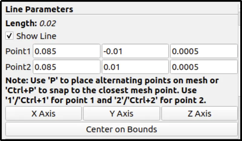
• Open simulation file in paraView and plot the velocity profile at point 0.085m from inlet.
• Repeat above procedure for grading factor 0.2 to check the differences in results.
• Write a detailed report explaining all the command and codes used in project.

Problem Statement:-

simulate an incompressible-laminar-viscous flow through the backward facing step geometry.

perform 2 case studies as described below and compare the results.

Case 1 - Simulate the flow without using any grading factor (i.e., GF = 1)

Case 2 - Simulate the flow with grading factor of 0.2. The cells should be finer near the walls (including the step wall).

Mesh specification:-

1. Number of cells along the x direction (longer dimension) = 200
2. Number of cells along the longer y direction = 20;

Boundary condition specification

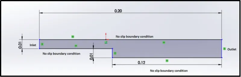
The domain specifications are provided in the following figure.

Theory:

Incompressible-laminar-viscous flow.

Incompressible flow:

The flow in which there is no change in the density is called the incompressible flow.

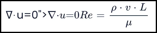
Mathematically, an incompressible flow can be expressed as

Laminar flow:

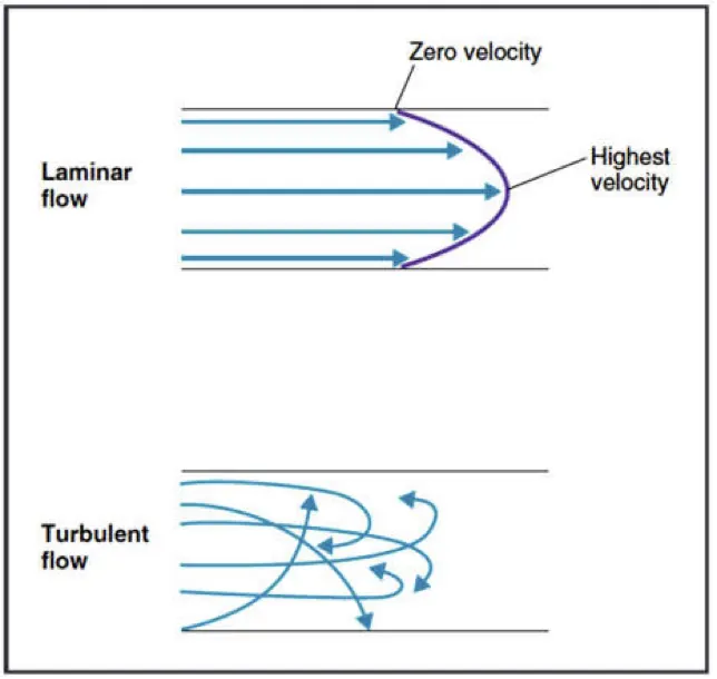
A laminar flow is one where the fluid motion is regular and there is no mixing. It can be visualised by the path lines that do not intersect each other.

In fluid dynamics, laminar flow is characterised by fluid particles following smooth paths in layers, with each layer moving smoothly past the adjacent layers with little or no mixing.

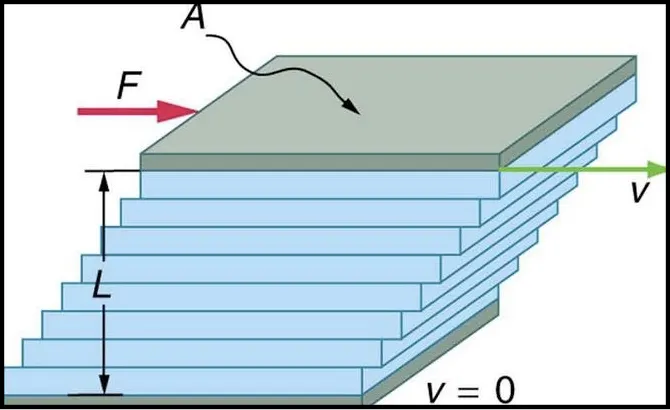
At low velocities, the fluid tends to flow without lateral mixing, and adjacent layers slide past one another like playing cards. There are no cross-currents perpendicular to the direction of flow, nor eddies or swirls of fluids.

In laminar flow, the motion of the particles of the fluid is very orderly with particles close to a solid surface moving in straight lines parallel to that surface. Laminar flow is a flow regime characterised by high momentum diffusion and low momentum convection.

Reynolds number is the parameter to differentiate a flow as laminar or turbulent.

Whenever the Reynolds number is less than about 2,000, flow in a pipe is generally laminar, whereas, at values greater than 2,000, flow is usually turbulent.

Mathematically, Reynolds number is the ratio of inertial force to the viscous force.

The Reynolds number is defined as

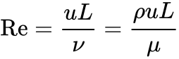
where:

• ρ is the density of the fluid (SI units: kg/m³)
• u is the flow speed (m/s)
• L is a characteristic linear dimension (m) (see the below sections of this article for examples)
• μ is the dynamic viscosity of the fluid (Pa·s or N·s/m² or kg/(m·s))
• ν is the kinematic viscosity of the fluid (m²/s).

Viscous flow.

A type of fluid flow in which there is a continuous steady motion of the particles; the motion at a fixed point always remains constant. Also called streamline flow; laminar flow; steady flow.

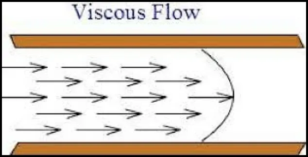
The fluid flow in form of a layer. The layer which sticks with the wall has zero velocity which is called no-slip condition and it develops the frictional effect at the wall. Frictional effects are also present between two layers of fluid and slower layer tries to slow down the faster layer which can be measured by using viscosity.

effects of viscosity are maximum near the boundary so laminar sublayer exists near the boundary that is shown in the below figure.

Mesh grading.

Mesh grading is a factor that is,

Grading factor = Size of the last cell / Size of the first cell

PROCEDURE.

• First, we are creating the run folder in OpenFOAM in which we will be running our simulations.
• And then need to copy the cavity folder to the run folder so that we can make the changes in the blockMeshDict, controlDict, and pressure and velocity files as to run our required simulations, we copying the folder because we are not supposed to make any changes in the original folders in the OpenFOAM.
• Then will make the required changes in the blockMeshDict file that is naming the vertices for and then creating the blocks, in this case, there are 21 vertices and 5 blocks while creating blocks we also need to specify the number of mesh points needed along the x, y, and z-direction and also the simple grading should be done along the boundaries.
• then, we need to assign the boundary conditions here, we need to define all the faces in OpenFOAM refers to patches and giving them type that is the inlet and outlet will be the faces (type patch), for front and back type will be empty faces, for top and bottom which are the boundary conditions in this case type will be wall type and setting up these will constitute a particular boundary, then will save these changes in the blockMeshDict.
• Then, in the velocity and pressure files, we have to give the value of the velocity at the inlet type will be fixed value here we should assign some value as initial velocity and pressure will be zero gradient and at the outlet velocity type will be zero gradient and pressure will be type fixed value that value will be uniform 0, then at front and back velocity type empty and pressure, as well as type empty at the no slip boundaries that is top and bottom velocity, will be type no slip and pressure type empty and in the transport properties, we can change the nu value in order to obtain the lower courant number.
• And in the controlDict file the simulation time and the time step need be assigned in the way that the courant number should be less than 0.5.
• and then creating the block mesh and then run the simulation using the respective solver after the completion of simulation open the paraview in the paraFoam and plot the velocity profile for the given value.

In order to start the simulation process, First start terminal xterm in XQuartz app .After starting XQuartz will see following window.

To operate openfoam need to login docker site.

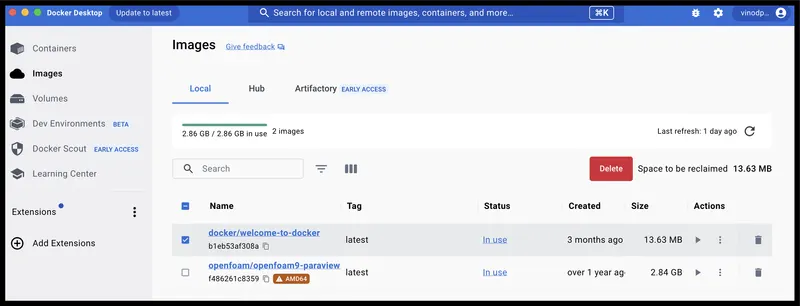
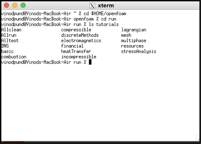
Now, we have to simulate our problem in openFOAM and we are going to solve our problem using tutorials present in openFOAM, therefore, just type commands on xterm terminal in sequence.

>>cd $HOME/openfoam

>>cd run

>>ls tutorials

To identify what kind of tutorials present inside this directory.

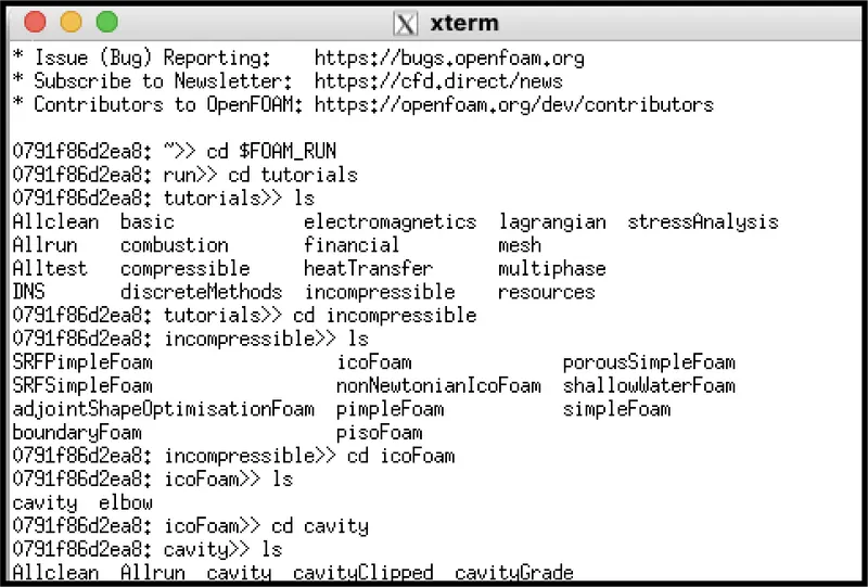
We have to solve incompressible flow simulation for this problem so select incompressible directory by typing ‘cd tutorials’ then ‘cd incompressible’ and then again type ls to explore folders in incompressible folders.

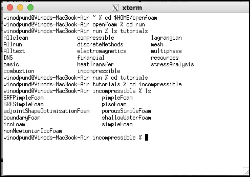
In above picture, we can see the plethora of solver folders. For this particular solver we need solver for laminar-viscous flow. So here we choose ‘icoFoam’

icoFoam is the solver in openFoam which is use as transient solver for incompressible, laminar flow of Newtonian fluids.

(Newtonian fluid is a fluid in which the viscous stress arising from its flow, at every point, are linearly correlated to the local strain rate - the rate of change of its deformation over time. Newtonian fluids are the simplest mathematical models of fluids that account for viscosity.)

Therefore, we will select icoFoam folder by typing ‘cd icoFoam’ and by typing ‘ls’ we explore this folder in terminal.

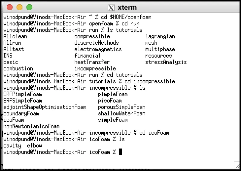
Here, we have, again to option, cavity and elbow. They both are part of the icoFoam solver and cavity section use to create required domain and black mesh so select ‘cavity’ folder.

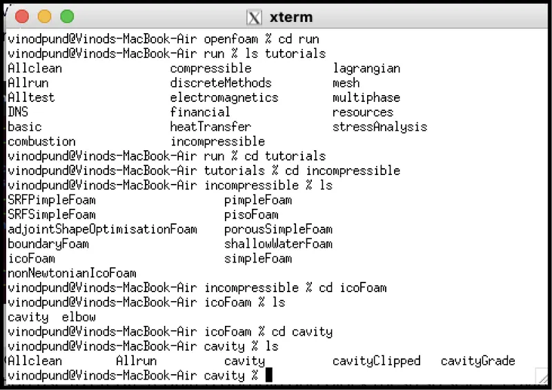
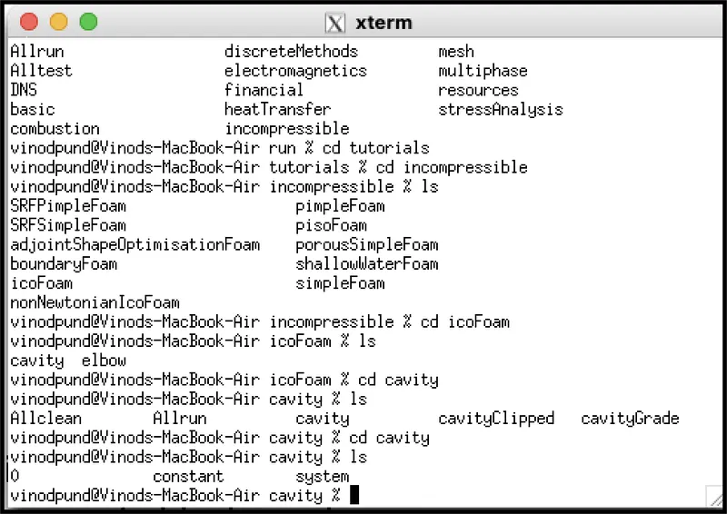
In cavity, we are, again, going to see cavity folder, where we have to define our fluid domain and generate block mesh.

But we are not going to make any changes here in tutorial section. First of all, OpenFoam does not let anyone make any changes in their official tutorial and secondly, any changes with their official tutorials my corrupt openFoam. An in a bid to correct it, we may need to reinstall open foam all over again.

So, we are going to copy this cavity folder using ‘cp -r cavity’ command and paste it in openFoam run folder by typing ‘cp -r cavity $FOAM_RUN/cavity_test’.

And then open run folder by typing ‘cd $FOAM_RUN’. where we can see cavity_test file.

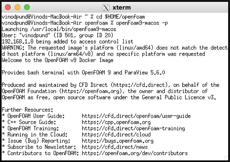
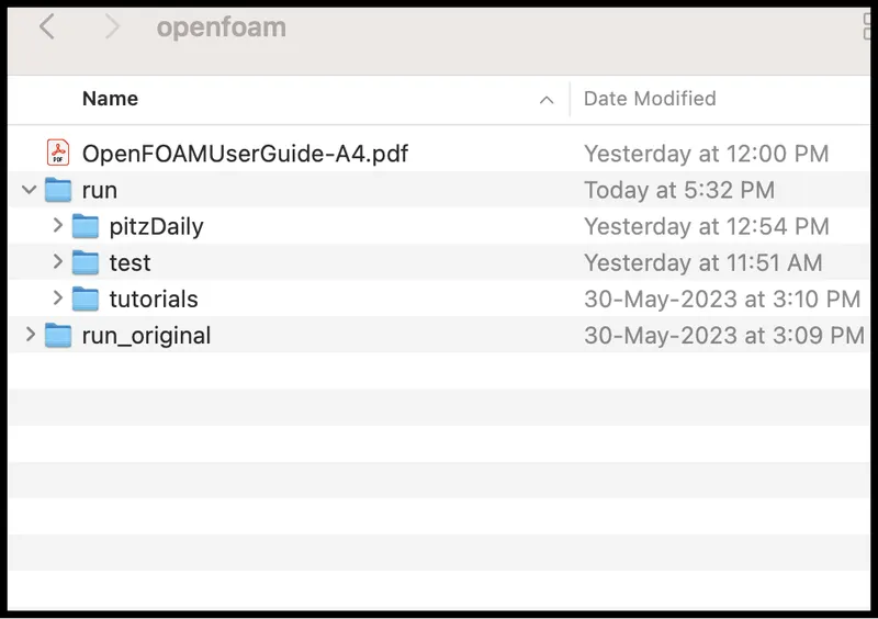
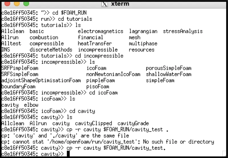
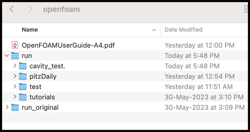
Command :- cp -r cavity $FOAM_RUN/cavity_test

Now, we can make any changes to the cavity_test file, which will never affect the openFoam official files. Open cavity_test folder. Here, we can provide specification for our block mesh in system folder.

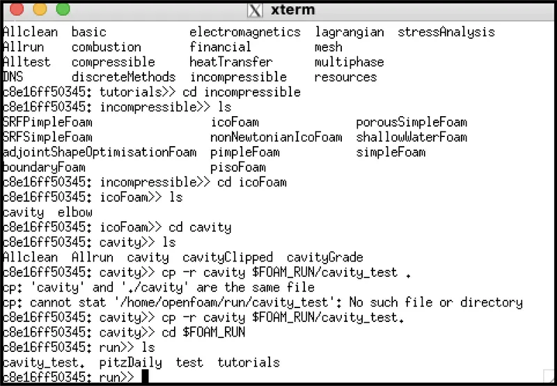
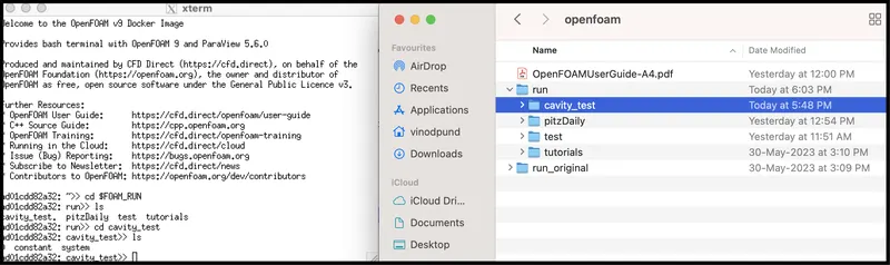
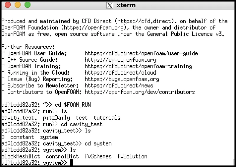
As we can see in above picture, there are 4 script file system folder and by opening blockMeshDict we can create domain and provide required specification for block mesh.So, open this file by typing ‘gedit blockMeshDict’.

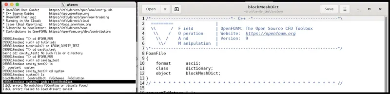
Now, make following changes in blockMeshDict script file.

The blockMeshDict file is a script file that contains information regarding all aspects of the geometry.

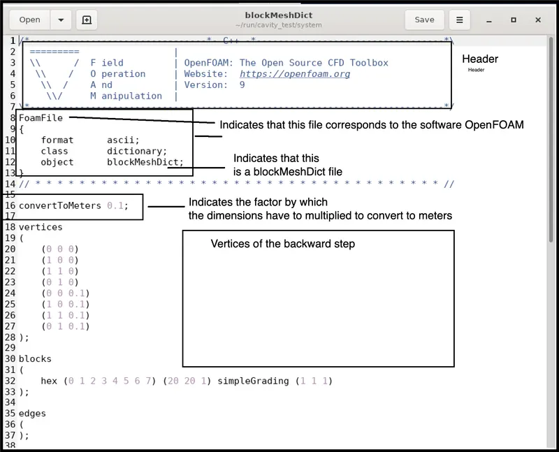
When you open this file, first, you are going to see header information in the form of comment which is not executable.

Next, we set units in meter, by converting all type of length in to meter.

convertToMeters 0.01;

Mesh generation without any grading factor

In the same blockMesh file go to the lines where we the word hex can be found. That is the line where we specify the faces of the blocks and also the number of cells in X, Y and Z direction.

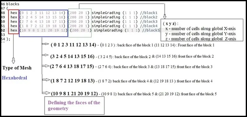
Also you specify the faces as the inlet, outlet and walls as shown in the picture below.

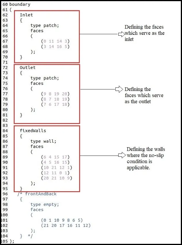
The blockMeshDict file is edited as shown in the above.

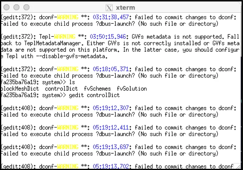
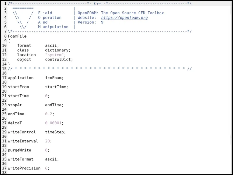
The next step is to navigate to the controlDict folder and specify the simulation time as 200 seconds.The script file looks as follows.

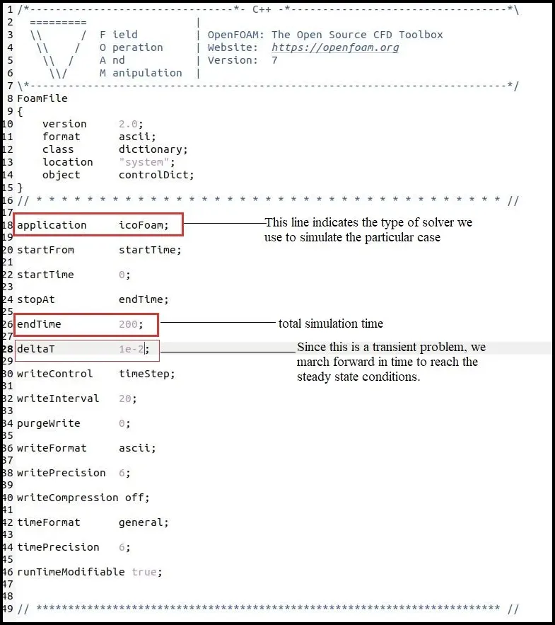
Vertices:-

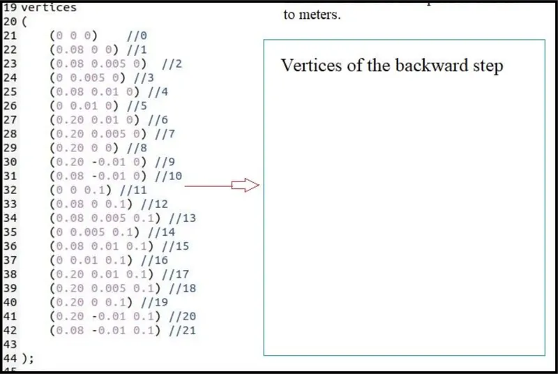
Afterward, in codes, we provide list of vertices by providing x, y and z coordinates locations; its always start from vertex (0,0,0). so we have to create following geometry.

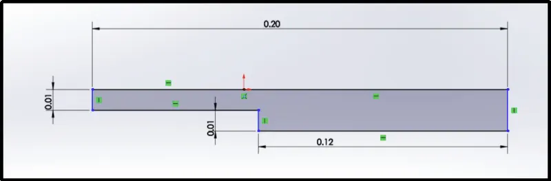
To create the above geometry, let us consider creating the geometry using 5 blocks as exhibited in below figure.

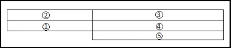
Now, you are going to provide vertices for each block by referring following sketch.

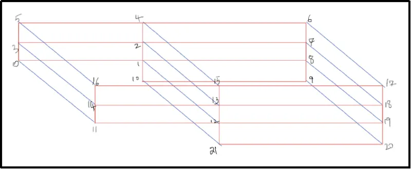
vertices

(

(0 0 0) //0

(8 0 0) //1

(8 0.5 0) //2

(0 0.5 0) //3

(8 1 0) //4

(0 1 0) //5

(20 1 0) //6

(20 0.5 0) //7

(20 0 0) //8

(20 -1 0) //9

(8 -1 0) //10

(0 0 0.1) //11

(8 0 0.1) //12

(8 0.5 0.1) //13

(0 0.5 0.1) //14

(8 1 0.1) //15

(0 1 0.1) //16

(20 1 0.1) //17

(20 0.5 0.1) //18

(20 0 0.1) //19

(20 -1 0.1) //20

(8 -1 0.1) //21

);

Next, we are going to define block for meshing. If we look at he mesh format first letter, in block parenthesis, is ‘hex’ which define type of mesh which is hexahedral mesh.

Then, again in parenthesis, we provide vertices number according to order which follow right hand thumb rule, meaning, thumb is the z axis and order of vertices follow rotational order of our other finger.

Then comes, number of mesh grid that we want to divide along x, y, and z length. We define it as (nx, ny, nz) format.

Given mesh specification:

1.Number of cells along the x direction(longer dimension) = 200

2.Number of cells along the longer y direction = 20

Lastly, we give simple grading which is cell expansion ratios

Grading factor or expansion ratios:-

The expansion ratios enables the mesh to be graded, or refined, in specified directions. The ratio is that of the width of the end cell δe along one edge of a block to the width of the start cell δs along the edge as shown in below figure.

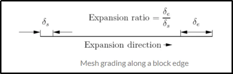
In simple format,

Expansion ratio = (size of end cell) / (size of starting cell)

The simple description specifies uniform expansion in the local x1, x2 and x3

directions respectively with only 3 expansion ratio. For first case, we are not going to provide any grading for our problem.

So here, we have 5 blocks so we have to define hex mesh for 5 blocks.

blocks

(

hex (0 1 2 3 11 12 13 14) (200 20 1) simpleGrading (1 1 1) // block1

hex (3 2 4 5 14 13 15 16) (200 20 1) simpleGrading (1 1 1) // block2

hex (2 7 6 4 13 18 17 15) (200 20 1) simpleGrading (1 1 1) // block3

hex (1 8 7 2 12 19 18 13) (200 20 1) simpleGrading (1 1 1) // block4

hex (10 9 8 1 21 20 19 12) (200 20 1) simpleGrading (1 1 1) // block5

);

Next, define boundary of the problem, in this we have to define faces of the our 3d block this should be in order according to right hand thumb rule. So set faces for this problem following way.

edges

(

);

boundary

(

inlet

{

type wall;

faces

(

(0 11 14 3)

(3 14 16 5)

);

}

outlet

{

type wall;

faces

(

(9 8 19 20)

(8 7 18 19)

(7 6 17 18)

);

}

frontAndBack

{

type empty;

faces

(

(11 12 13 14)

(14 13 15 16)

(13 18 17 15)

(12 19 18 13)

(21 20 19 12)

(0 3 2 1)

(3 5 4 2)

(2 4 6 7)

(1 2 7 8)

(10 1 8 9)

);

}

fixedWalls

{

type wall;

faces

(

(5 16 15 4)

(0 1 12 11)

(4 15 17 6)

(10 9 20 21)

(10 21 12 1)

);

}

);

mergePatchPairs

(

);

// ************************************************************************* //

After, editing of blockMeshDic file save it and close it.

Edit codes following way

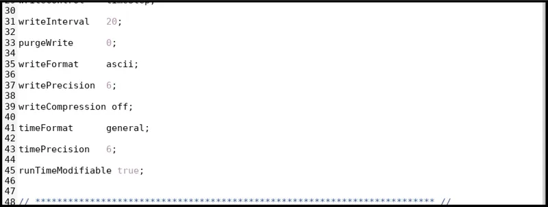
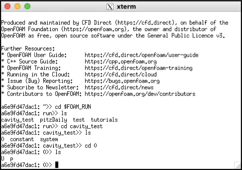
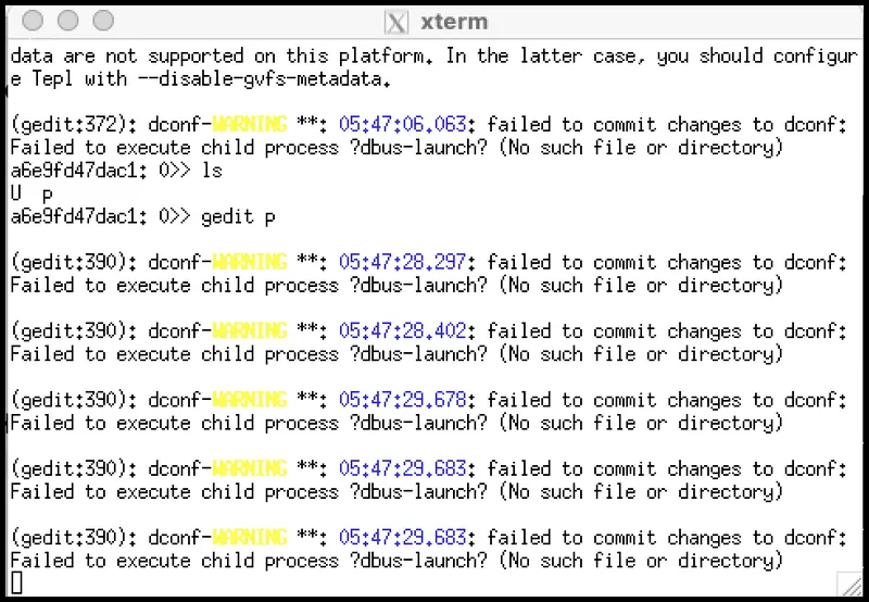
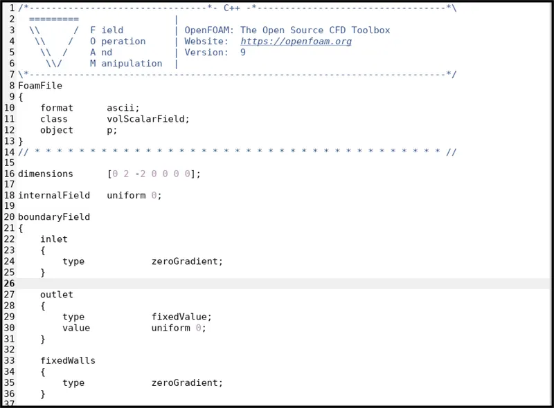
Then, you have to define initial value for pressure and velocity. In order to do that, you have to go back in cavity_test directory using ‘cd 0’ command and select folder named ‘0’, which stand for initial values. In this case initial value for pressure and velocity.

In this case, we have to set initial boundary condition for pressure and velocity at each faces also update the name of the boundary same as you changed inlet outlet name in ‘blockMeshDict’ script file as per shown in below codes.

Initial setting for Velocity

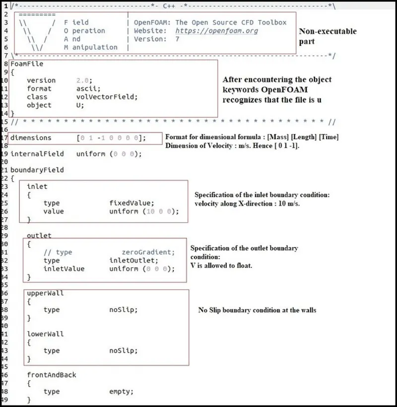
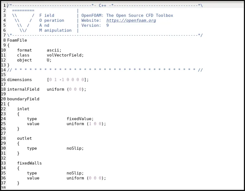
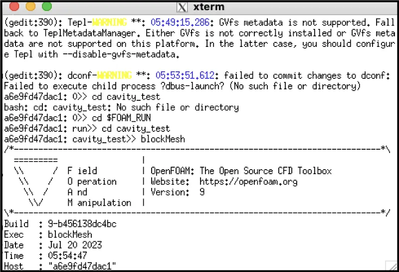
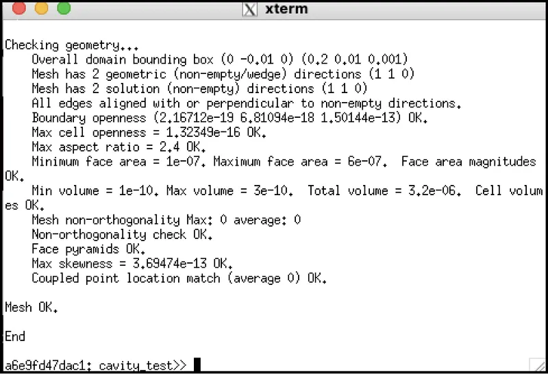
At this point, our problem statement is set, we can now proceed to deploy mesh using ‘blockMesh’ command and then use ‘checkMesh’ command to check if there any error in our mesh.

blockMesh

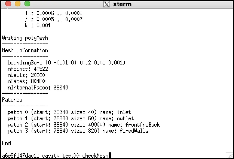
After, checking mesh we get following confirmation

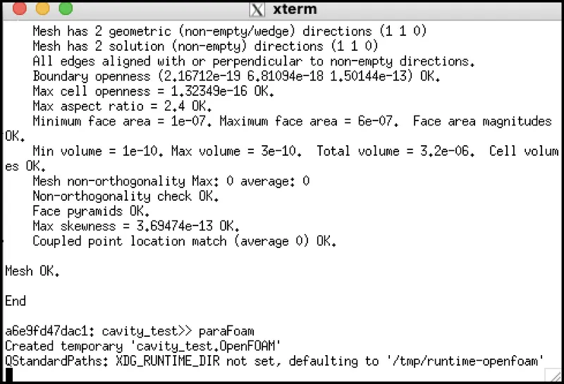
At this stage, we can check our mesh is as per requirement or not by using paraView typing paraFoam command.

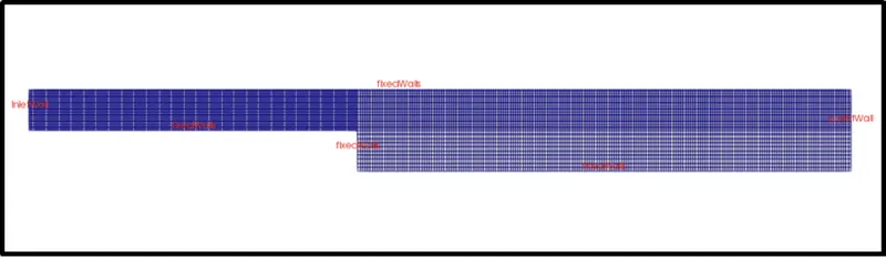
Take a look at above mesh. One can notice it is not uniform all over the surface. So let us just adjust the mesh grid following way.

hex (0 1 2 3 11 12 13 14) (80 5 1) simpleGrading (1 1 1) // block1

hex (3 2 4 5 14 13 15 16) (80 5 1) simpleGrading (1 1 1) // block2

hex (2 7 6 4 13 18 17 15) (120 5 1) simpleGrading (1 1 1) // block3

hex (1 8 7 2 12 19 18 13) (120 5 1) simpleGrading (1 1 1) // block4

hex (10 9 8 1 21 20 19 12) (120 10 1) simpleGrading (1 1 1) // block5

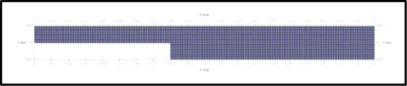
After making above changes, now the mesh is uniformly distributed along the surface.

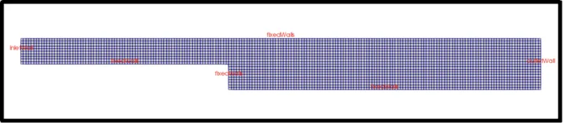
After deploying mesh, now we are ready to run the simulation. Simulation that we selected was icoFoam. Hence, just type ‘icoFoam’ and simulation will start.

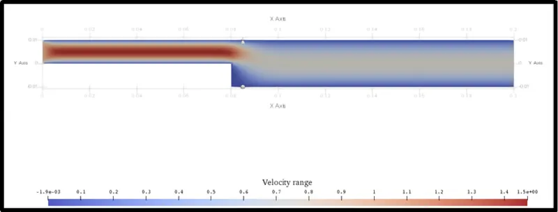
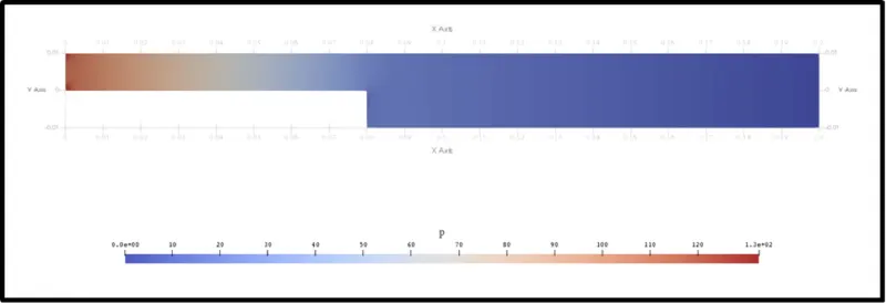
Now, let us view the results in paraView by using ‘paraFoam’ command

Mesh grid:-

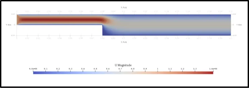
Velocity Distribution along the domain area:-

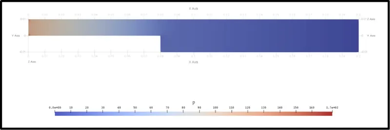
Pressure Distribution along the domain area:-

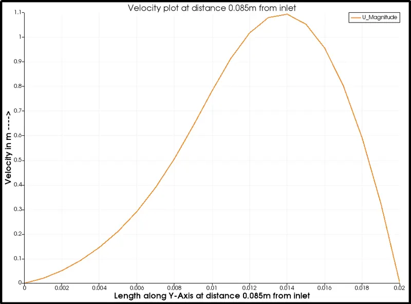
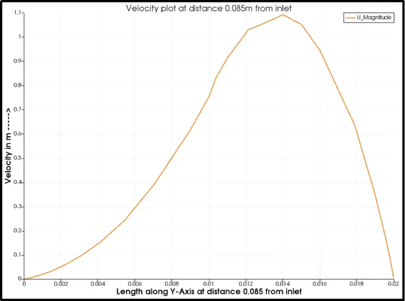
To Calculate velocity at distance 0.085 from inlet modify following parameters.

Velocity Plot:-

With Grading Factor 0.2 (cell near fixed walls)

Now, lets solve same problem for grading factor 0.2

blocks

(

hex (0 1 2 3 11 12 13 14) (80 5 1) simpleGrading (0.2 5 1) // block1 (1/0.2) = 5

hex (3 2 4 5 14 13 15 16) (80 5 1) simpleGrading (0.2 0.2 1) // block2

hex (2 7 6 4 13 18 17 15) (120 5 1) simpleGrading (5 0.2 1) // block3 (1/0.2) = 5

hex (1 8 7 2 12 19 18 13) (120 5 1) simpleGrading (5 5 1) // block4 (1/0.2) = 5

hex (10 9 8 1 21 20 19 12) (120 10 1) simpleGrading (5 5 1) // block5 (1/0.2) = 5

);

Output mesh from above codes:-

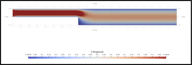
Velocity Distribution along the domain area:-

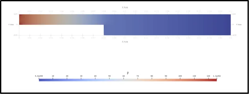
Pressure Distribution along the domain area:-

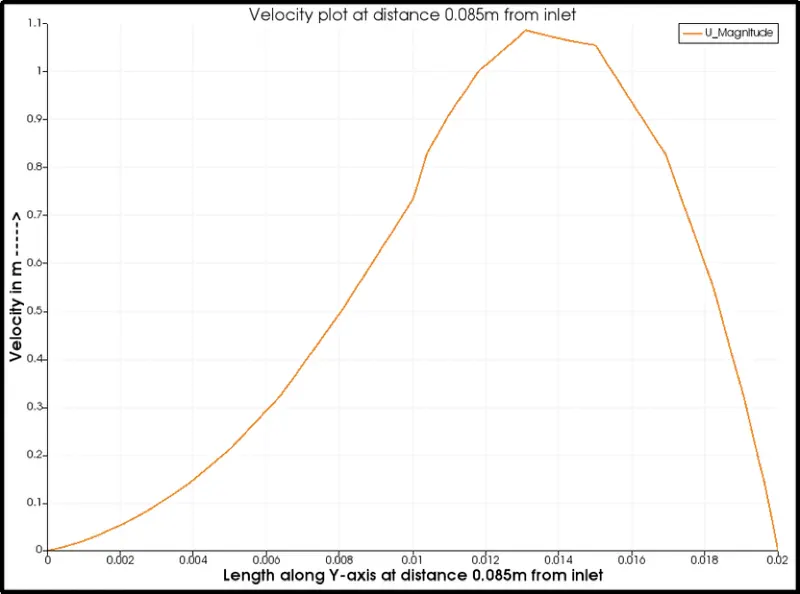
Velocity Plot:-

With Grading Factor 0.2 (cell near All walls)

Next, use grading factor 0.2 for all walls in the system.

blocks

(

hex (0 1 2 3 11 12 13 14) (80 5 1) // block1

simpleGrading

(

(

(0.5 0.5 5) // 50% y-dir, 50% cells, expansion = 5

(0.5 0.5 0.2) // 50% y-dir, 50% cells, expansion = 0.2 (1/5)

)

(

(0.8 0.9 5) // 80% y-dir, 90% cells, expansion = 5

(0.2 0.1 1) // 20% y-dir, 10% cells, expansion = 1

)

1 // z-direction expansion ratio

)

hex (3 2 4 5 14 13 15 16) (80 5 1) // block2

simpleGrading

(

(

(0.5 0.5 5) // 50% y-dir, 50% cells, expansion = 5

(0.5 0.5 0.2) // 50% y-dir, 50% cells, expansion = 0.2 (1/5)

)

(

(0.2 0.1 1) // 20% y-dir, 10% cells, expansion = 1

(0.8 0.9 0.2) // 80% y-dir, 90% cells, expansion = 5

)

1 // z-direction expansion ratio

)

hex (2 7 6 4 13 18 17 15) (120 5 1) // block3

simpleGrading

(

(

(0.5 0.5 5) // 50% y-dir, 50% cells, expansion = 5

(0.5 0.5 0.2) // 50% y-dir, 50% cells, expansion = 0.2 (1/5)

)

(

(0.2 0.1 1) // 20% y-dir, 10% cells, expansion = 1

(0.8 0.9 0.2) // 80% y-dir, 90% cells, expansion = 5

)

1 // z-direction expansion ratio

)

hex (1 8 7 2 12 19 18 13) (120 5 1) // block4

simpleGrading

(

(

(0.5 0.5 5) // 50% y-dir, 50% cells, expansion = 5

(0.5 0.5 0.2) // 50% y-dir, 50% cells, expansion = 0.2 (1/5)

)

(

(0.8 0.9 5) // 80% y-dir, 90% cells, expansion = 5

(0.2 0.1 1) // 20% y-dir, 10% cells, expansion = 1

)

1 // z-direction expansion ratio

)

hex (10 9 8 1 21 20 19 12) (120 10 1) // block5

simpleGrading

(

(

(0.5 0.5 5) // 50% y-dir, 50% cells, expansion = 5

(0.5 0.5 0.2) // 50% y-dir, 50% cells, expansion = 0.2 (1/5)

)

(

(0.9 0.9 5) // 90% y-dir, 90% cells, expansion = 5

(0.1 0.1 1) // 10% y-dir, 10% cells, expansion = 1

)

1 // z-direction expansion ratio

)

);

Output mesh from above codes:-

Velocity Distribution along the domain area:-

Velocity Distribution along the domain area:-

Pressure Distribution along the domain area:-

Velocity Plot:-

Results

- Up to this point, we have done plotting velocity plot for both, without grading factor and with 0.2 grading factor, cases. If we take a look at all the three line graph, we can see, the plot for velocity without grading factor seems more smooth and accurate than other two plot. So one can say, grading can disrupt out result. But it is incorrect. Because, if we take good look at it, we can notice, the mesh is fine at step wall along the X-axis but very coarse along Y-axis. Therefore, we are not getting smooth plot for velocity at 0.085 point at Y-axis.

- To understand this thing clearly, we can see below figure, where we can see- on the left side there is coarse mesh and on the right side fine mesh. Above picture, there respective graphs are presented, which can really convince anyone how at any given point mesh produce a plot. The one on the right side mesh is giving very smooth plot except one small pick near point 0.01 and on the other hand, for coarse structured mesh, the curve of graph the curve is not smooth, there are sharp corner forming at the top of the curve.

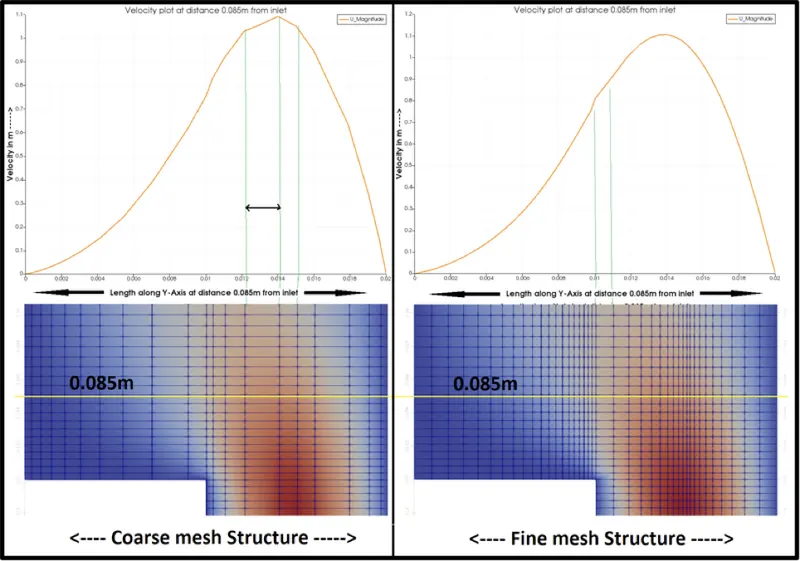
- After learning how mesh actually works, we should use fine mesh near the point where we expect our results. In CFD fluid always shows large changes near walls and obstacles along its way and to capture those changes effectively we should always use grading or finer mesh near a wall.

- To get effective and reliable results, one should know where to use finer grading factor. In a bid to obtain more effective results, suppose, if we use large number of fine elements, it could use our computation time and also require large computational memory(RAM). Therefore, use of grading is important, so that, we can use fine mesh to capture the flow at boundary wall and obstacles, course mesh at more open area.

- We can also see importance of fine mesh by observing following picture. As grading factor increasing near step, the resolution of image in improving. Means, as the number of element is increasing, the flow result is also increasing.

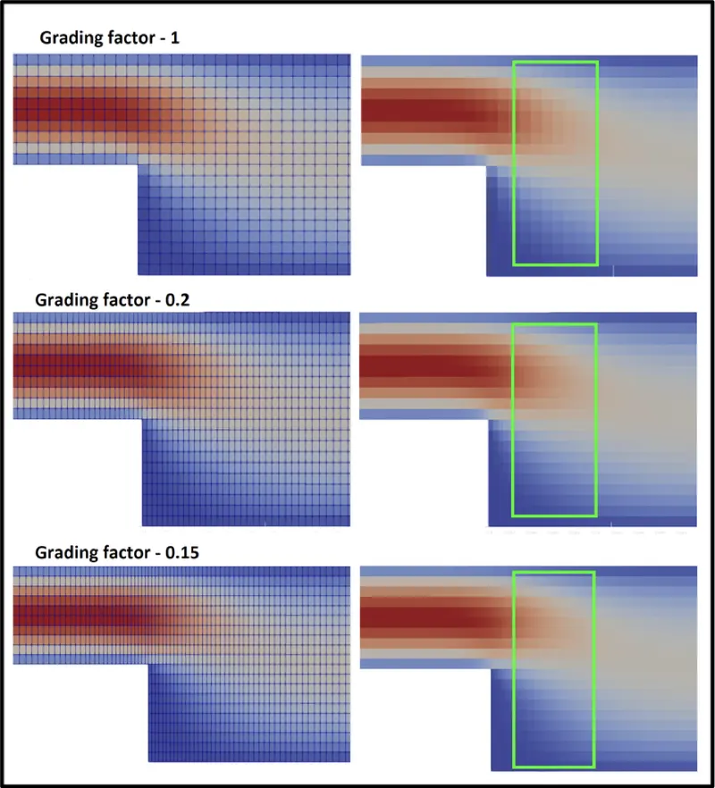
- We can see more fine result at grading factor 0.15. Hence, always use fine mesh in the area where maximum changes happen in velocity, pressure or other property of fluid, to capture more detailed and accurate results.

CONCLUSION.

By changing the simple grading factor from the value of 0.2 to 1 the mesh becomes finer and the solution becomes very accurate.

Overall the change in the size of simple grading factor (mesh size) the results remains the same as approximately.

The execution time is lower for lower meshing grading factor.