Week 8 - Simulation of a backward facing step in OpenFOAM
Title : Simulation of a backward facing step in OpenFOAM
Aim / Objectives :
- simulate an incompressible-laminar-viscous flow through the backward facing step geometry
- Perform transient simulation
- Select solver based on the physics of the flow described in the problem statement.
- Explanation of simulation process and way of setting up the problem statement in openFOAM
- Explain every changes that we have done inside the reference case files obtained from OpenFOAM tutorials.
- Next, preform two case study, firstly simulation of the flow without using any grading factor (i.e., GF = 1) and secondly simulate the flow with grading factor of 0.2.
Introduction
In the field of computational fluid dynamics, one of the interesting problem is the Backward Facing Step (BFS) problem. The OpenFOAM package is used to perform two-dimensional numerical simulations of laminar backward-facing step flow in this project. Open-source post-processing software ParaView is used to produce a mesh using the OpenFoam software and to display the changes in velocity and pressure gradients for a given mesh grading factor. The icoFoam solver-based transient analysis of our computational flow is included in this report.
Theory (BACKWARD FACING STEP)
Backward-Facing Step (BFS) flow is one representative separation-flow model, which is of significance in both theoretical and engineering development. Various applications for BFS flow can be found in our daily life, such as the airfoils at large attack angle, the spoiler flows, separation flow behind a vehicle, inlet tunnel flow of engine also the flow around a boat or a building.
Backward-Facing Step (BFS) has also been partially discussed in general previous studies of flow separation dynamics. The flow separation after a simple stage will introduce separation bubble formation, evolution and re-attachment process, which is dependent on the BFS geometric design, the inlet and outlet conditions , etc...
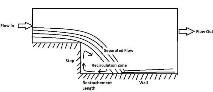
Mesh specification
- Number of cells along the x direction (longer dimension) = 200
- Number of cells along the longer y direction = 20;
The domain specifications are provided in the following figure.
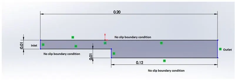
STEPS TO SIMULATE THIS PARTICULAR PROBLEM IN OPENFOAM
In order to start the simulation process, first we have to launch Terminal. Now, we have to simulate our problem in openFOAM and we are going to solve our problem using tutorials present in openFOAM, therefore, just type ‘tut’ to open OpenFOAM tutorial directory. And type ‘ls’ to identify what kind of tutorials present inside this directory.

As this is a problem of incompressible laminar viscous flow so select incompressible directory by typing ‘cd incompressible’ and then again type ls to explore folders inside incompressible folders.

For this particular solver we need solver for laminar-viscous flow. So here we choose ‘icoFoam’ .
IcoFoam is the solver present in openfoam. This is Transient solver for incompressible, laminar flow of Newtonian fluids. icoFoam solves the incompressible laminar Navier-Stokes equations using the PISO algorithm.
PISO : The PISO (Pressure Implicit with Splitting of Operators) is an efficient method to solve the Navier-Stokes equations in unsteady problems.
So now, we will select icoFoam folder by typing ‘cd icoFoam’ and by typing ‘ls’ we explore this folder in terminal.

Here, we can see that inside icoFoam solver there is cavity and again inside cavity there is one more cavity and elbow option. Cavity section is used to create the geometry domain and blockmesh so select ‘cavity’ folder.
So, now inorder to explor we will go inside cavity typing 'cd cavity' and 'ls'.

Here, we can see inside the cavity folder there is three option 0, constant and system. Now, we will copy this cavity folder in openfoam run folder and inside this run folder we will run all our simulation.
So, now by typing 'cp -r cavity/ $FOAM_RUN/test' we are going to copy cavity folder and paste it run folder and rename it as test.
And , then we will open our folder section by typing 'explorer.exe .'
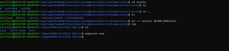
Now, we can make any changes to the test file, which will never affect the openFoam official file. Here, we can provide specification for our block mesh in system folder.
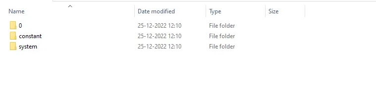
Now, here we can see that inside the cavity folder (test) we have three option. The directory 0 contains boundary conditions (BC) and initial conditions (IC) P and U.
The directory constant contains physical properties. Inside the system directory , there is four more folder which is blockMeshDict, controlDict, fvSchemes and fvSolutions.
GEOMETRY and MESH GENERATION
Now, to create our desired geometry, we are going to divide our domain into five individual blocks, it will give us the ease to change our geometry according to our mesh grading factor. The domain is divided into five blocks with respective vertices, as shown below:
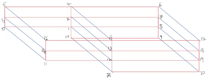
Now, we will make following changes in blockMeshDict script file. To create geometry and to generate a mesh in OpenFOAM, we need to edit the BlockMeshDict file; it can be found under the system folder of our case tutorial ("cavity," in this case)
The blockMeshDict file is a script file that contains information regarding all aspects of the geometry (vertices, blocks, mesh information, boundary, etc..)
blockMeshDict:(Gradient factor of 1)
/*--------------------------------*- C++ -*----------------------------------*\
  =========                 |
  \\      /  F ield         | OpenFOAM: The Open Source CFD Toolbox
   \\    /   O peration     | Website:  https://openfoam.org
    \\  /    A nd           | Version:  10
     \\/     M anipulation  |
\*---------------------------------------------------------------------------*/
FoamFile
{
    format      ascii;
    class       dictionary;
    object      blockMeshDict;
}
// * * * * * * * * * * * * * * * * * * * * * * * * * * * * * * * * * * * * * //

convertToMeters 1;

vertices
(
    (0 0 0)            //0
    (0.08 0 0)         //1
    (0.08 0.005 0)     //2
    (0 0.005 0)        //3
    (0.08 0.01 0)      //4
    (0 0.01 0)         //5
    (0.2 0.01 0)       //6
    (0.2 0.005 0)      //7
    (0.2 0 0)          //8
    (0.2 -0.01 0)      //9
    (0.08 -0.01 0)     //10
    (0 0 0.1)          //11
    (0.08 0 0.1)       //12
    (0.08 0.005 0.1)   //13
    (0 0.005 0.1)      //14
    (0.08 0.01 0.1)    //15
    (0 0.01 0.1)       //16
    (0.2 0.01 0.1)     //17
    (0.2 0.005 0.1)    //18
    (0.2 0 0.1)        //19
    (0.2 -0.01 0.1)    //20
    (0.08 -0.01 0.1)   //21

);

blocks
(
    hex (0 1 2 3 11 12 13 14) (80 5 1) simpleGrading (1 1 1)
    hex (3 2 4 5 14 13 15 16) (80 5 1) simpleGrading (1 1 1)
    hex (2 7 6 4 13 18 17 15) (120 5 1) simpleGrading (1 1 1)
    hex (1 8 7 2 12 19 18 13) (120 5 1) simpleGrading (1 1 1)
    hex (10 9 8 1 21 20 19 12) (120 10 1) simpleGrading (1 1 1)
);

boundary
(
    inlet
    {
        type patch;
        faces
        (
            (0 11 14 3)
            (3 14 16 5)
        );
    }
    outlet
    {
        type patch;
        faces
        (
            (9 8 19 20)
            (8 7 18 19)
            (7 6 17 18)
        );
    }
    frontAndBack
    {
        type empty;
        faces
        (
            (0 3 2 1)
            (3 5 4 2)
            (1 2 7 8)
            (2 4 6 7)
            (10 1 8 9)
            (11 12 13 14)
            (14 13 15 16)
            (13 18 17 15)
            (12 19 18 13)
            (21 20 19 12)
        );
    }
    noslipwall
    {
        type wall;
        faces
        (
            (4 5 16 15)
            (4 15 17 6)
            (0 1 12 11)
            (9 20 21 10)
            (1 10 21 12)

        );
    }
);
mergePatchpairs
(
);


// ************************************************************************* //
The blockMeshDict file is edited as shown in the above ans save it.
Now, we are going to edit ‘controlDict’ file to provides time limits - start time and end time timestep size. After edting save it and close it.
controlDict file
/*--------------------------------*- C++ -*----------------------------------*\
  =========                 |
  \\      /  F ield         | OpenFOAM: The Open Source CFD Toolbox
   \\    /   O peration     | Website:  https://openfoam.org
    \\  /    A nd           | Version:  10
     \\/     M anipulation  |
\*---------------------------------------------------------------------------*/
FoamFile
{
    format      ascii;
    class       dictionary;
    location    "system";
    object      controlDict;
}
// * * * * * * * * * * * * * * * * * * * * * * * * * * * * * * * * * * * * * //

application     icoFoam;

startFrom       startTime;

startTime       0;

stopAt          endTime;

endTime         0.2;

deltaT          0.00001;

writeControl    timeStep;

writeInterval   10;

purgeWrite      0;

writeFormat     ascii;

writePrecision  6;

writeCompression off;

timeFormat      general;

timePrecision   6;

runTimeModifiable true;


// ************************************************************************* //
Specifying physical properties
In OpenFOAM, the physical parameters for a specific flow problem are described in the file called physicalProperties file. This file is located in the constant directory under our case file. In our case, we have assumed that our fluid is a Newtonian fluid, and the kinematic viscosity of fluid flow is given as 0.01 m^2/second.
The respective TphysicalProperties file is written below(this file will be the same for all analysis with different grading factor) :
/*--------------------------------*- C++ -*----------------------------------*\
  =========                 |
  \\      /  F ield         | OpenFOAM: The Open Source CFD Toolbox
   \\    /   O peration     | Website:  https://openfoam.org
    \\  /    A nd           | Version:  10
     \\/     M anipulation  |
\*---------------------------------------------------------------------------*/
FoamFile
{
    format      ascii;
    class       dictionary;
    location    "constant";
    object      physicalProperties;
}
// * * * * * * * * * * * * * * * * * * * * * * * * * * * * * * * * * * * * * //

nu              [0 2 -1 0 0 0 0] 0.01;


// ************************************************************************* //
Giving Initial and Boundary conditions
Governing equations are the same for every CFD problem, and then there should be something that makes our results unique for every flow problem. This is done by Boundary conditions which are unique for every CFD problem. We can specify our inlet-velocity and outlet-pressure condition in the respective notepad file located inside the 0 folder in our run-case directory.
Next, we have to set initial boundary condition for pressure and velocity at each faces also update the name of the boundary same as we changed inlet outlet name in ‘blockMeshDict’ script file as per shown in below codes.
Initial and boundary condition for Pressure
/*--------------------------------*- C++ -*----------------------------------*\
  =========                 |
  \\      /  F ield         | OpenFOAM: The Open Source CFD Toolbox
   \\    /   O peration     | Website:  https://openfoam.org
    \\  /    A nd           | Version:  10
     \\/     M anipulation  |
\*---------------------------------------------------------------------------*/
FoamFile
{
    format      ascii;
    class       volScalarField;
    object      p;
}
// * * * * * * * * * * * * * * * * * * * * * * * * * * * * * * * * * * * * * //

dimensions      [0 2 -2 0 0 0 0];

internalField   uniform 0;

boundaryField
{
    inlet
    {
        type            zeroGradient;
    }

    outlet
    {
        type            fixedValue;
        value           uniform 0;
    }

    noslipwall
    {
        type            zeroGradient;
    }

    frontAndBack
    {
        type            empty;
    }
}

// ************************************************************************* //
Initial and boundary condition for Velocity
/*--------------------------------*- C++ -*----------------------------------*\
  =========                 |
  \\      /  F ield         | OpenFOAM: The Open Source CFD Toolbox
   \\    /   O peration     | Website:  https://openfoam.org
    \\  /    A nd           | Version:  10
     \\/     M anipulation  |
\*---------------------------------------------------------------------------*/
FoamFile
{
    format      ascii;
    class       volVectorField;
    object      U;
}
// * * * * * * * * * * * * * * * * * * * * * * * * * * * * * * * * * * * * * //

dimensions      [0 1 -1 0 0 0 0];

internalField   uniform (0 0 0);

boundaryField
{
    inlet
    {
        type            fixedValue;
        value           uniform (0.2 0 0);
    }

    outlet
    {
        type            zeroGradient;
    }

    noslipwall
    {
        type            noSlip;
    }

    frontAndBack
    {
        type            empty;
    }
}

// ************************************************************************* //
Our problem is set. Now, we will come back to terminal and will run the blockMesh and checkMesh to check our generate mesh, is it ok or there is any errror.
After running , we got following confirmation from openFoam.
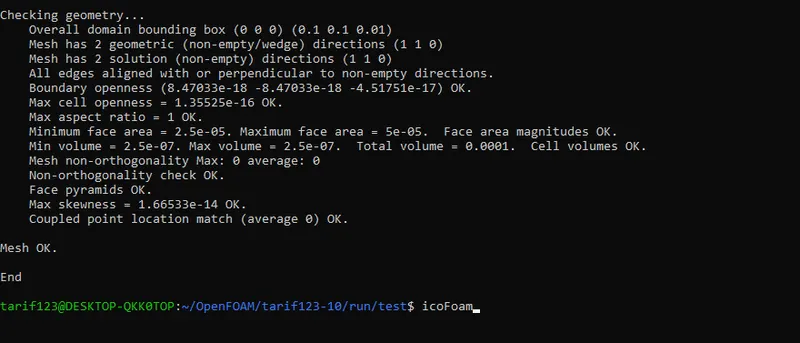
Now we will launch paraview inorder to view our generate mesh . Inorder to open paraview type 'touch result.foam' and then type 'explorer.exe .' Now by visiting the run/test/result folder we can launch the paraview.

Mesh grid
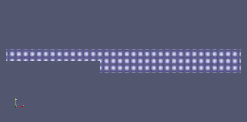
You can see that, all over the domain cell size is uniform because we have meshed the geometry without grading factor ( GF = Size of end cell / size of start cell = 1)
After deploying mesh, now we are ready to run the simulation. Simulation that we selected was icoFoam. Hence, just type ‘icoFoam’ and simulation will start.
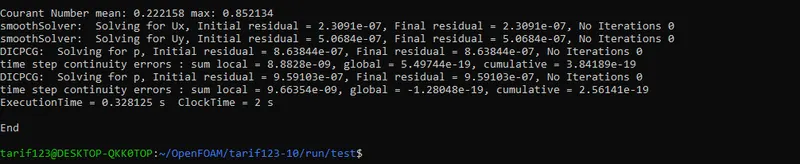
Now again go to paraview we have already opened it and view the result.
Case 1 (GF = 1)
Mesh grid
- Number of cells along the x direction (longer dimension) = 200
- Number of cells along the longer y direction = 20
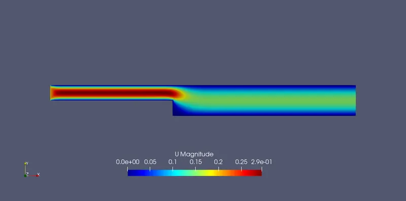
Velocity distribution along the domain
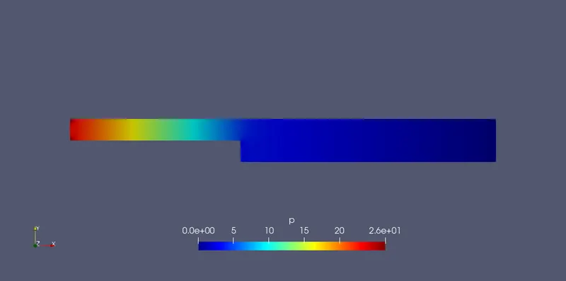
Pressure distribution along the domain
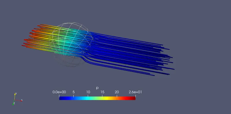
Visualization of pressure distribution using streamtube
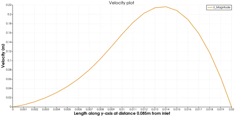
Velocity profile at 0.085 m from the inlet of the geometry
Case 2 (GF = 0.2)
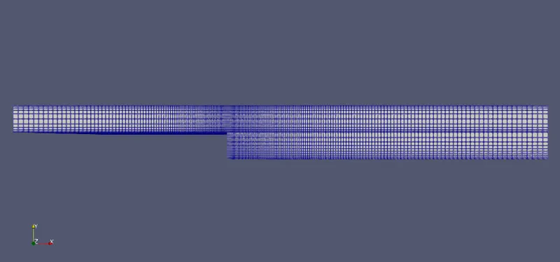
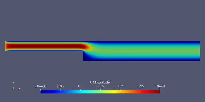
For this case , we are interested to see the velocity distribution. So, we will refine the mesh near the wall to capture more information at this location.
WE have made the following changes in blockMeshDict file for grading factor 0.2.
blocks
(
    hex (0 1 2 3 11 12 13 14) (80 5 1) simpleGrading (0.2 5 1)    //block1
    hex (3 2 4 5 14 13 15 16) (80 5 1) simpleGrading (0.2 0.2 1)  //block2
    hex (2 7 6 4 13 18 17 15) (120 5 1) simpleGrading (5 0.2 1)   //block3
    hex (1 8 7 2 12 19 18 13) (120 5 1) simpleGrading (5 5 1)     //block4
    hex (10 9 8 1 21 20 19 12) (120 10 1) simpleGrading (5 5 1)   //block5
);
Complete blockMeshDict file for Grading factor = 0.2
/*--------------------------------*- C++ -*----------------------------------*\
  =========                 |
  \\      /  F ield         | OpenFOAM: The Open Source CFD Toolbox
   \\    /   O peration     | Website:  https://openfoam.org
    \\  /    A nd           | Version:  10
     \\/     M anipulation  |
\*---------------------------------------------------------------------------*/
FoamFile
{
    format      ascii;
    class       dictionary;
    object      blockMeshDict;
}
// * * * * * * * * * * * * * * * * * * * * * * * * * * * * * * * * * * * * * //

convertToMeters 1;

vertices
(
    (0 0 0)            //0
    (0.08 0 0)         //1
    (0.08 0.005 0)     //2
    (0 0.005 0)        //3
    (0.08 0.01 0)      //4
    (0 0.01 0)         //5
    (0.2 0.01 0)       //6
    (0.2 0.005 0)      //7
    (0.2 0 0)          //8
    (0.2 -0.01 0)      //9
    (0.08 -0.01 0)     //10
    (0 0 0.1)          //11
    (0.08 0 0.1)       //12
    (0.08 0.005 0.1)   //13
    (0 0.005 0.1)      //14
    (0.08 0.01 0.1)    //15
    (0 0.01 0.1)       //16
    (0.2 0.01 0.1)     //17
    (0.2 0.005 0.1)    //18
    (0.2 0 0.1)        //19
    (0.2 -0.01 0.1)    //20
    (0.08 -0.01 0.1)   //21

);

blocks
(
    hex (0 1 2 3 11 12 13 14) (80 5 1) simpleGrading (0.2 5 1)    //block1
    hex (3 2 4 5 14 13 15 16) (80 5 1) simpleGrading (0.2 0.2 1)  //block2
    hex (2 7 6 4 13 18 17 15) (120 5 1) simpleGrading (5 0.2 1)   //block3
    hex (1 8 7 2 12 19 18 13) (120 5 1) simpleGrading (5 5 1)     //block4
    hex (10 9 8 1 21 20 19 12) (120 10 1) simpleGrading (5 5 1)   //block5
);

boundary
(
    inlet
    {
        type patch;
        faces
        (
            (0 11 14 3)
            (3 14 16 5)
        );
    }
    outlet
    {
        type patch;
        faces
        (
            (9 8 19 20)
            (8 7 18 19)
            (7 6 17 18)
        );
    }
    frontAndBack
    {
        type empty;
        faces
        (
            (0 3 2 1)
            (3 5 4 2)
            (1 2 7 8)
            (2 4 6 7)
            (10 1 8 9)
            (11 12 13 14)
            (14 13 15 16)
            (13 18 17 15)
            (12 19 18 13)
            (21 20 19 12)
        );
    }
    noslipwall
    {
        type wall;
        faces
        (
            (4 5 16 15)
            (4 15 17 6)
            (0 1 12 11)
            (9 20 21 10)
            (1 10 21 12)

        );
    }
);
mergePatchpairs
(
);


// ************************************************************************* //
Mesh grid with GF = 0.2
controlDict file
In OpenFOAM, input data relating to the control of time and reading and writing of the solution data are read in from the controlDict dictionary.
/*--------------------------------*- C++ -*----------------------------------*\
  =========                 |
  \\      /  F ield         | OpenFOAM: The Open Source CFD Toolbox
   \\    /   O peration     | Website:  https://openfoam.org
    \\  /    A nd           | Version:  10
     \\/     M anipulation  |
\*---------------------------------------------------------------------------*/
FoamFile
{
    format      ascii;
    class       dictionary;
    location    "system";
    object      controlDict;
}
// * * * * * * * * * * * * * * * * * * * * * * * * * * * * * * * * * * * * * //

application     icoFoam;

startFrom       startTime;

startTime       0;

stopAt          endTime;

endTime         0.2;

deltaT          0.00001;

writeControl    timeStep;

writeInterval   10;

purgeWrite      0;

writeFormat     ascii;

writePrecision  6;

writeCompression off;

timeFormat      general;

timePrecision   6;

runTimeModifiable true;


// ************************************************************************* //
Giving Initial and Boundary conditions
Governing equations are the same for every CFD problem, and then there should be something that makes our results unique for every flow problem. This is done by Boundary conditions which are unique for every CFD problem. We can specify our inlet-velocity and outlet-pressure condition in the respective notepad file located inside the 0 folder in our run-case directory.
Initial and boundary conditions for Velocity
/*--------------------------------*- C++ -*----------------------------------*\
  =========                 |
  \\      /  F ield         | OpenFOAM: The Open Source CFD Toolbox
   \\    /   O peration     | Website:  https://openfoam.org
    \\  /    A nd           | Version:  10
     \\/     M anipulation  |
\*---------------------------------------------------------------------------*/
FoamFile
{
    format      ascii;
    class       volVectorField;
    object      U;
}
// * * * * * * * * * * * * * * * * * * * * * * * * * * * * * * * * * * * * * //

dimensions      [0 1 -1 0 0 0 0];

internalField   uniform (0 0 0);

boundaryField
{
    inlet
    {
        type            fixedValue;
        value           uniform (0.2 0 0);
    }

    outlet
    {
        type            zeroGradient;
    }

    noslipwall
    {
        type            noSlip;
    }

    frontAndBack
    {
        type            empty;
    }
}

// ************************************************************************* //
Initial and boundary conditions for Pressure
/*--------------------------------*- C++ -*----------------------------------*\
  =========                 |
  \\      /  F ield         | OpenFOAM: The Open Source CFD Toolbox
   \\    /   O peration     | Website:  https://openfoam.org
    \\  /    A nd           | Version:  10
     \\/     M anipulation  |
\*---------------------------------------------------------------------------*/
FoamFile
{
    format      ascii;
    class       volScalarField;
    object      p;
}
// * * * * * * * * * * * * * * * * * * * * * * * * * * * * * * * * * * * * * //

dimensions      [0 2 -2 0 0 0 0];

internalField   uniform 0;

boundaryField
{
    inlet
    {
        type            zeroGradient;
    }

    outlet
    {
        type            fixedValue;
        value           uniform 0;
    }

    noslipwall
    {
        type            zeroGradient;
    }

    frontAndBack
    {
        type            empty;
    }
}

// ************************************************************************* //
Results
Velocity distribution along the domain
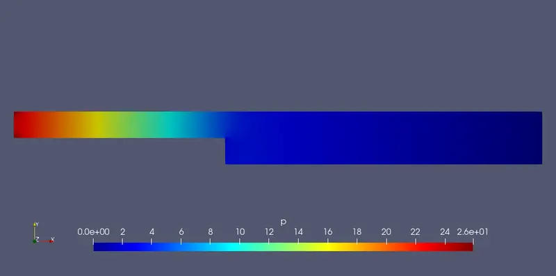
Pressure distribution along the domain
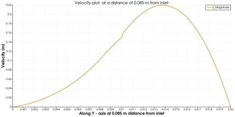
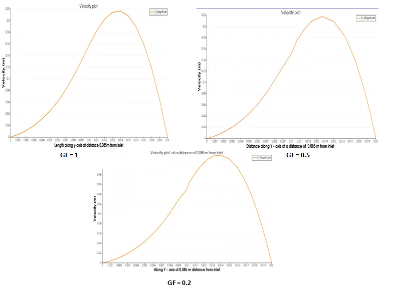
Velocity profile at 0.085 m from the inlet of the geometry
Comparison of velocity plot :
Observations :
- Due to the small geometry and low velocity, grading has no effect on flow behavior.
- The effects of the wall boundary layer are effectively captured by grading.
- The velocity curves are slightly distorted because the middle of the grading mesh is coarse.
- The area is pretty smooth throughout the curve that was obtained without grading the mesh.
- We should have finer mesh near the walls for better results, and among all the mesh generated in this , the mesh with a grading factor of 0.2 provides us with the finest mesh near the walls.
Conslusions :
- So, we have successfully simulated the transient simulation of 2 D laminar flow over backward facing step geometry using openFOAM.
- We have performed 2 case studies by making the changes in blockmeshdict file . One is without grading factor and second is with grading factor and compared the velocity profile with each other
- The velocity graphs obtained from the different meshing grading factors are similar except negligible variations. As the mesh's cell size is smaller, i.e., for finer mesh, we can visualize the accurate output.
- After Plotting the velocity graph at a distance of 0.085 m from inlet along Y - axis, it can be seen that the velocity at the walls is zero, whereas the velocity at the center is maximum. This is due to the no-slip boundary condition at the walls .i.e. velocity at the walls is zero.
- Further, similar plots can be seen for different grading points without further change. However, it can be said that the finer mesh can lead to better accuracy of the results.
References :
1. Lin Chen et al.
A review of Backward - Facing Step(BFS) flow mechanism, heat transfer and control (2018)