Week 8 - Simulation of a backward facing step in OpenFOAM
AIM : To simulate incompressible laminar viscous flow over a backward facing step using OpenFOAM and compare the results obtained from different meshes.
THEORY :
Incompressible flow : It is a type of flow in which the density of the fluid is taken to be constant. Therefore its derivative with respect to both time and space is 0
`(∂ρ)/(∂t) = (∂ρ)/(∂x) = (∂ρ)/(∂y) = (∂ρ)/(∂z) = 0`
Viscous flow : A type of flow wherein resistive forces exist between adjacent layers. This resistive force is in the form of shear stresses, which progressively increase as the the streamlines (layer of fluid in laminar flow) move further away from the boundary.
`τ = μ (dv)/dy`; where `μ` is the dynamic viscosity, `v` the velocity and `y` the vertical distance
Laminar flow : Laminar flow is flow charactersied by low velocity and high viscocity. In this the fluid flows in the form of strealines. Laminar flow has a Reynold's number <= 2000.
`R_e = (ρ v L)/μ` ; where `R_e` is Reynolds number, `L` is characteristic Length
Backward Facing Step :
The significance of the simulation :
- Flow over a backward facing step has been used as a benchmarking and validation test for several numerical solutions. This is due to the step conviniently replicating the separation and subsequent recombination of flow and the ample availability of data.
- As the fluid reaches the step, an expansion of the flow channel results in a pressure gradient. This ultimately leads to the boundary layers separating from the flow. Whent the fluid reaches the bottom wall, the detached flow recombines, thus forming a loop of sorts.
- This phenomenon of separation and recombination prevails in systems like diffusers, combustion engine or flow around an airfoil etc.
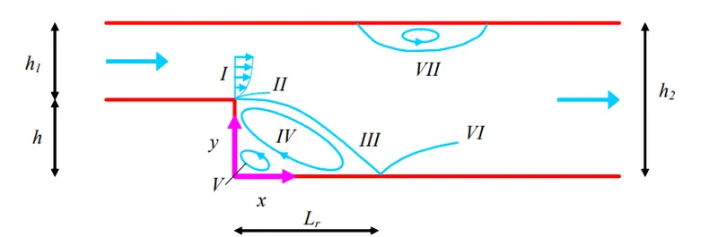
Fig 1 Schematic representation of the system
There are 7 regions of interest in the system highlighted as shown above[1].
- (I) inlet boundary
- (II) separated free shear region
- (III) region of reattatchment
- (IV) primary recirculation region
- (V) corner recirculation region
- (VI) redevoloping boundary layer
- (VII) secondary separation region
Even though these regions have been mentioned, we aren't going to delve into their detail in this project.
Equations : In this simulation, only the Navier Stoke's equations,ie. the equations of continuity and conservation of momentum come into play. Further, the Z direction has not been taken into account, therby making the simulation 2 Dimensional.
Equation of continuity
`(∂ρ)/(∂t) + ▽ ρU = 0`
- Since flow is incompressible
`▽ U = 0`
`(∂u)/(∂x) + (∂v)/(∂y) = 0`
Conservation of Momentum
`ρ(Du)/(Dt) = -(∂P)/(∂x) + μ▽^2 u`
`ρ((∂u)/(∂t) + U*▽u) = -(∂P)/(∂x) + μ▽^2 u`
- Since u is the velocity along x direction
`ρ((∂u)/(∂t) + u(∂u)/(∂x) ) = -(∂P)/(∂x) + μ▽^2 u`
- Similarly in the y direction
`ρ((∂v)/(∂t) + v(∂v)/(∂y) ) = -(∂P)/(∂y) + μ▽^2 v`
SIMULATION:
Block Mesh
The simulation process begins with creating the blockmesh for the system. The blockmesh is made in the blockMeshDict file present in the 'system' directory of the simulation.
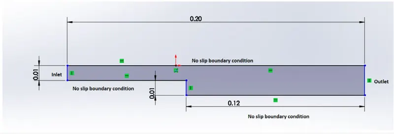
Fig. 2 System specifications
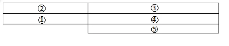
Fig. 3 Dividing the system into blocks
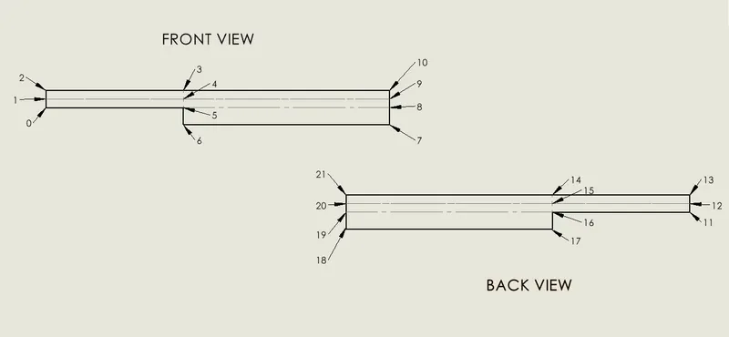
Fig. 4 The vertices of the blockmesh
blockMeshDict file
/*--------------------------------*- C++ -*----------------------------------*
  =========                 |
        /  F ield         | OpenFOAM: The Open Source CFD Toolbox
       /   O peration     | Website:  https://openfoam.org
      /    A nd           | Version:  10
     /     M anipulation  |
*---------------------------------------------------------------------------*/
FoamFile
{
    format      ascii;
    class       dictionary;
    object      blockMeshDict;
}
// * * * * * * * * * * * * * * * * * * * * * * * * * * * * * * * * * * * * * //

convertToMeters 1; // since the dimensions are already provided in meters

vertices
(
    (0 0 0.005) //0
    (0 0.005 0.005) //1
    (0 0.01 0.005) //2
    (0.08 0.01 0.005) //3
    (0.08 0.005 0.005) //4
    (0.08 0 0.005) //5
    (0.08 -0.01 0.005) //6
    (0.2 -0.01 0.005) //7
    (0.2 0 0.005) //8
    (0.2 0.005 0.005) //9
    (0.2 0.01 0.005) //10

    (0 0 -0.005) //11
    (0 0.005 -0.005) //12
    (0 0.01 -0.005) //13
    (0.08 0.01 -0.005) //14
    (0.08 0.005 -0.005)//15
    (0.08 0 -0.005) //16
    (0.08 -0.01 -0.005)//17
    (0.2 -0.01 -0.005) //18
    (0.2 0 -0.005) //19
    (0.2 0.005 -0.005) //20
    (0.2 0.01 -0.005) //21
);


blocks
(
    // 0.01 m = 10 cells


    //in the presence of grading

    /*hex (11 16 15 12 0 5 4 1) (80 5 1) simpleGrading (0.2 0.2 1)

    hex (12 15 14 13 1 4 3 2) (80 5 1) simpleGrading (0.2 0.2 1)

    hex (15 20 21 14 4 9 10 3) (120 5 1) simpleGrading (0.2 0.2 1)

    hex (16 19 20 15 5 8 9 4) (120 5 1) simpleGrading (0.2 0.2 1)

    hex (17 18 19 16 6 7 8 5) (120 10 1) simpleGrading (0.2 0.2 1)*/

    // in the absence of grading

    hex (11 16 15 12 0 5 4 1) (80 5 1) simpleGrading (1 1 1)

    hex (12 15 14 13 1 4 3 2) (80 5 1) simpleGrading (1 1 1)

    hex (15 20 21 14 4 9 10 3) (120 5 1) simpleGrading (1 1 1)

    hex (16 19 20 15 5 8 9 4) (120 5 1) simpleGrading (1 1 1)

    hex (17 18 19 16 6 7 8 5) (120 10 1) simpleGrading (1 1 1)
);

boundary
(
    inlet
    {
        type patch;
        faces
        (
            (0 1 12 11)
            (1 2 13 12)
        );
    }
    outlet
    {
        type patch;
        faces
        (
            (20 21 10 9)
            (19 20 9 8)
            (18 19 8 7)

        );
    }
    Wall //keyword used for wlls having noSlip conditio
    {
        type noSlip; //adhering to the no slip boundary condition
        faces
        (
            (2 3 14 13)
            (3 10 21 14)
            (16 5 0 11)
            (5 16 17 6)
            (18 7 6 17)

        );
    }
    frontAndBack
    {
        type empty;
        faces
        (
            (0 5 4 1)
            (1 4 3 2)
            (4 9 10 3)
            (5 8 9 4)
            (6 7 8 5)
            (12 15 16 11)
            (13 14 15 12)
            (14 21 20 15)
            (15 20 19 16)
            (16 19 18 17)
        );
    }
);

mergePatchPairs
(
);


// ************************************************************************* //
The list of vertices for a block is an ordered pair, ie. the vertices have to be mentioned in a specific order. 8 vertices make up a hexahedral block, 4 belonging to one face and the other 4 belonging to the opposite face.
The list of vertices can be divided into 2 sets for the sake of convinience. The first set of vertices belonging to one face, and the second set belonging to the opposite one.
- In each set, there are 3 pairs of vertices
- The first pair of vertices must signify the direction of x-axis
- The second pair of vertices signify the Y-axis
- The third pair is again along the x direction
Therefore in almost every case, it will be the Front and Back faces of the hexahedron which are taken into consideration
It has been observed that the vertices ofthe Back face have to mentioned first, followed by the Front face.
Taking block 1 as an example, made from vertices 0 1 4 5 11 12 15 16.
- The vertices of the Back Face are ordered as (11 16 15 12)
- Pair (11 16) signify x direction, (16 15) signifies Y direction, (15 12) brings it back along the x axis
- Similarly in the Front Face, the order is (0 5 4 1)
- Thus the list of vertices for Block 1 is (11 16 15 12 0 5 4 1).
Input/Output operations & Solver
The I/O operations of the simulation are present in the controlDict file of the system directory.
Since we intend to create a transient simulation for an incompressible laminar Newtonian Fluid, the icoFoam solver has been used to solve the equations mentioned above.
controlDict file
/*--------------------------------*- C++ -*----------------------------------*
  =========                 |
        /  F ield         | OpenFOAM: The Open Source CFD Toolbox
       /   O peration     | Website:  https://openfoam.org
      /    A nd           | Version:  10
     /     M anipulation  |
*---------------------------------------------------------------------------*/
FoamFile
{
    format      ascii;
    class       dictionary;
    location    "system";
    object      controlDict;
}
// * * * * * * * * * * * * * * * * * * * * * * * * * * * * * * * * * * * * * //

application     icoFoam; // does not supporttransient flow?

startFrom       startTime;

startTime       0;

stopAt          endTime;

endTime         1;

deltaT          0.0001;

writeControl    timeStep;

writeInterval   1000; // to write data at progressions of 0.1 delta T

purgeWrite      0;

writeFormat     ascii;

writePrecision  6;

writeCompression off;

timeFormat      general;

timePrecision   6;

runTimeModifiable true;


// ************************************************************************* //
Boundary Conditions
Boundary conditions are set in 0 directory of the simulation, which indicates the initial time step of the simulation. The conditions to keep in mind are
- Simulate a Laminar flow
- Apply boundary conditions to the blocks as indicated in Fig. 2
Simulating Laminar flow : In order to simulate Laminar flow, the Reynold's number `R_e` should be < 2000. For the purpose of this simulation, the inlet velocity `U_(mean)` is taken to be `30 m//s`. The kinematic viscosity `v` (pnew) is taken to be `0.01 m^2//s` . The characteristic length `L` is taken as the length of the step, ie `0.2 m`. At the outlet a constant static pressure of `P = 0` has been assumed. The value of outlet velocity is extrapolated using nearby cells.
Kinematic velocity present in the physicalProperties file of the 'constant' directory
/*--------------------------------*- C++ -*----------------------------------*
  =========                 |
        /  F ield         | OpenFOAM: The Open Source CFD Toolbox
       /   O peration     | Website:  https://openfoam.org
      /    A nd           | Version:  10
     /     M anipulation  |
*---------------------------------------------------------------------------*/
FoamFile
{
    format      ascii;
    class       dictionary;
    location    "constant";
    object      physicalProperties;
}
// * * * * * * * * * * * * * * * * * * * * * * * * * * * * * * * * * * * * * //

nu              [0 2 -1 0 0 0 0] 0.01;


// ************************************************************************* //
Boundary Conditions for `U`
/*--------------------------------*- C++ -*----------------------------------*
  =========                 |
        /  F ield         | OpenFOAM: The Open Source CFD Toolbox
       /   O peration     | Website:  https://openfoam.org
      /    A nd           | Version:  10
     /     M anipulation  |
*---------------------------------------------------------------------------*/
FoamFile
{
    format      ascii;
    class       volVectorField;
    object      U;
}
// * * * * * * * * * * * * * * * * * * * * * * * * * * * * * * * * * * * * * //

dimensions      [0 1 -1 0 0 0 0];

internalField   uniform (0 0 0);

boundaryField
{
    inlet
    {
        type            fixedValue;
        value           uniform (30 0 0); // inlet velocity of 30
    }

    outlet
    {
        type            zeroGradient; //to extrpolate from nearby cells

    }

    Wall
    {
        type            noSlip; //noSlip boundary condition
    }

    frontAndBack
    {
        type            empty;
    }
}

// ************************************************************************* //
Boundary conditions for `P`
/*--------------------------------*- C++ -*----------------------------------*
  =========                 |
        /  F ield         | OpenFOAM: The Open Source CFD Toolbox
       /   O peration     | Website:  https://openfoam.org
      /    A nd           | Version:  10
     /     M anipulation  |
*---------------------------------------------------------------------------*/
FoamFile
{
    format      ascii;
    class       volScalarField;
    object      p;
}
// * * * * * * * * * * * * * * * * * * * * * * * * * * * * * * * * * * * * * //

dimensions      [0 2 -2 0 0 0 0];

internalField   uniform 0;

boundaryField
{
    inlet
    {
        type            zeroGradient;
    }

    outlet
    {
        type            fixedValue;
        value           uniform 0;
    }

    Wall
    {
        type            zeroGradient;
    }

    frontAndBack
    {
        type            empty;
    }
}

// ************************************************************************* //
OBSERVATIONS :
The observations have been divided based on the presence or absence of grading in the Block Mesh. Grading is the practice of varying the cell size in a mesh in order to augment the results. The Grading Factor (GF) is defined as the ratio of the size of end cell to the first cell.
The Pressure profile of the fluid across the system
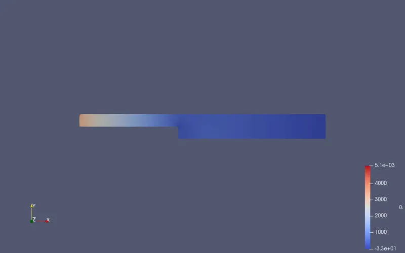
Fig. 5 Pressure distribution
Velocity Profile of the fluid across the system
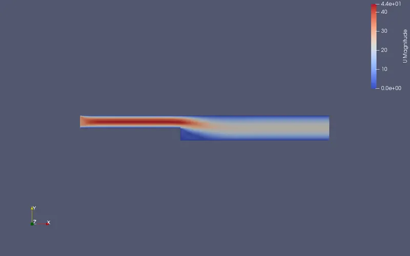
Fig 6 Velocity distribution
Case 1: GF = 1
The velocity profile shown with the help of streamlines with the Tube and Glyph filter
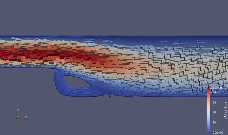
Fig. 7 Ungraded velocity profile
Velocity profile at the region of separation, `x = 0.085m`
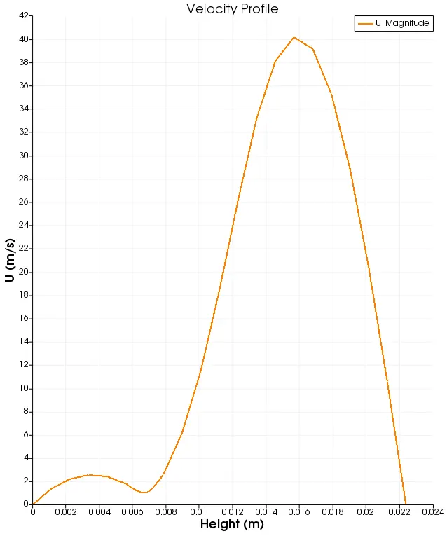
Fig. 8 The velocity profile at region II
Case 2) : GF = 0.2
The velocity profile shown with the help of streamlines with the Tube and Glyph filter
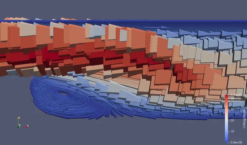
Fig. 9 Graded velocity profile
Velocity profile at the region of separation, `x = 0.085m`
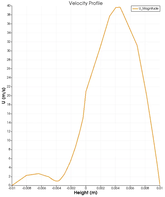
Fig. 10 The velocity profile at region II
In both the cases, the recirculation of the streamlines (curved lines tangential to the velocity profile at the point) are clearly visible in the primary recirculation region (IV), followed by the subsequent re-attatchment at region III .
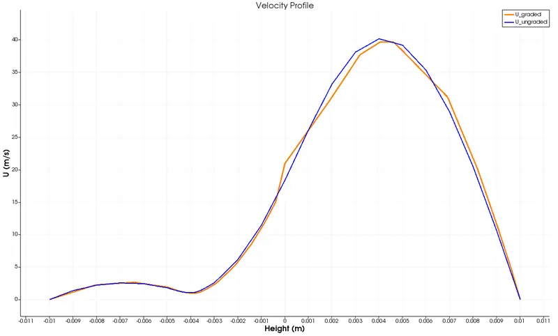
Fig. 11 Comparison of the velocity profile
It can be seen that, although minor, there are certain deviations in the velocity profile of the ungraded and graded simulation
In order to further study the affects of grading, the velocity profile over the entire region of recirculation (IV) has been considered. From `( 0.1,-0.01,0.005)` to `(0.081,-0.0005,0.005)` . A resolution of 150 has been chosen for the plot.
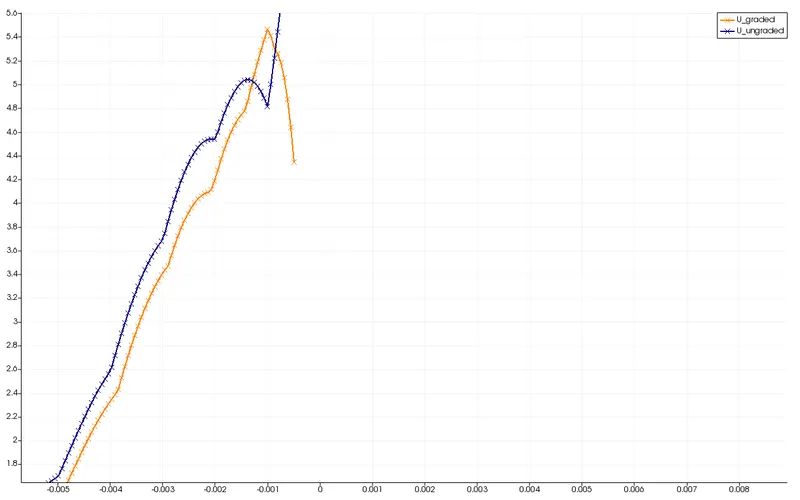
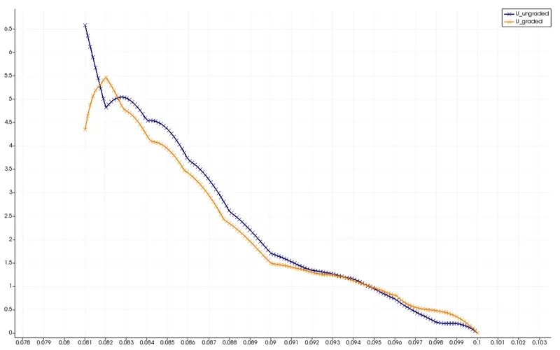
Fig. 12 Velocity profile across the height Fig. 13 Velocity Profile across the length
It is clearly seen that in the ungraded Mesh, there is linearity in parts of the profile whereas no such linearity prevails in the the graded mesh.
For the sake of testing, another mesh with a GF of 5 and 0.2 along the x and y- axis respectively is considered. This was done so that the region of interest (region IV) has the finest mesh possible.
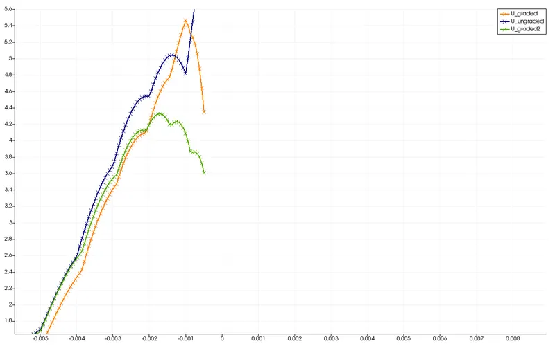
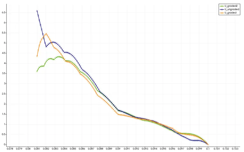
Fig. 14 Velocity profile across the height Fig. 15 Velocity Profile across the length
It can be seen that even linearities present in mesh with a uniform 2 D grading of 0.2 has been eliminated with the new GF.
INFERENCE:
- Grading makes the mesh finer, which makes for more accurate approximations
- Interpolating values during plots etc result in minimal error since the values at adjacent nodes are comparable in value
- Choosing a `GF > 1` or `GF < 1` depends on the region under speculation. There is no hard and fast rule for which provides a more accurate result
Bibliography