Week 11 - Simulation of Flow through a pipe in OpenFoam
AIM : To simulate flow through a pipe of circular crossection in OPENFOAM and verify the results using numerical solution of the same.
THEORY : Flow through a pipe is a common engineering problem which is applicable to several household and industrial requirements such as, water supply, transportation of checmicals, fuel etc. The reason flow through a pipe is generally simulated is to i) Analyze the pressure difference required to ensure steady flow ii) Set the dimension( diameter and length) required for steady flow iii) Optimise the flow by reducing major (friction) losses and minor losses (expansion, bends, entry, exit etc.).
However in this simulation we will solely to analyse incompressible, laminar flow of a real fluid through a pipe of desirered diameter and corresponding length.
The list of variables are -
`rho=`density;`P=`pressure;`w=`velocity(along z axis); `tau =`shear stress; `R =`radius of pipe; `Q =` volumetric flow rate; `nu`= kinematic viscocity;`mu=`dynamic viscocity; `R_e =`Reynold's number; `e =`energy
Incompressible : Flow is said to be incompressible when the density of the fluid is constant. Its derivative with respect to space and time is 0.
`(delrho)/(delt)=(delrho)/(delx)=(delrho)/(dely)=(delrho)/(delz)=0`
Laminar : A flow is said to be laminar if the streamlines of the fluid are parallel to one another. A non dimensional quantity called Reunold's number is used to indicate wheather a flow is laminar or turbulent. If
`R_e < 2000`; laminar flow
`2000ltR_elt4000`; transitional flow
`R_e>4000`; turbulent flow
Laminar flow is possible only for highly viscous and flows with relatively low speed
Viscocity : Viscocity is the friction offered to the flow of a fluid caused due to its veloicty gradient. It is responsible to the shear stress acting on a fluid. `tau = mu(dv)/(dy)`
Entrance length of pipe : Contrary to general practise, the entire length of a pipe does not have fully developed flow. For a certain length, the velocity profile changes as the length increases, i.e. it does not have its usual parabolic profile with velocity maximum at the centre and minimum at the edges. This length of the pipe is called entrance length(`L_e`). In the case of laminar flow
`L_e/D = 0.06R_e` ; where `D =`diameter
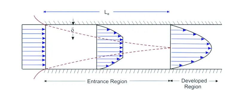
The figure shows the development of the boundary layer, i.e regions under the action of viscocity. It is vividly seen that at the inlet, the entire crossection has a common velocity, indicating the absence of a boundary layer. As the flow continues, under the action of shear stresses, the boundary layer thickens until it finally converges at the centre. That is where the flow becomes fully developed.
Reynold's number : Reynold's number of a flow is given by `R_e = (VD)/nu`, where `V`is the average velocity of the flow. Therefore as the velocity of the flow increases, it can change from laminar to turbulent. `
Pressure drop : A fluid always flows from a region of higher to lower pressure. The pressure gradient along the length of a pipe is required to keep a fluid flowing. It is analogous to the potential different across a circuit which is required to keep current flowing. The pressure gradient is given by Hagen Pouselli's equation
`triangleP = (8muLQ)/(piR^4)`; where `L` is length of the pipe
It should be noted that this pressure drop is applied only to the region of fully developed flow. As the length of the pipe increases, the shear stresses continue to act on it. However, we know that the velocity profile does not change in the fully developed region. In order to maintain this, we need a pressure gradient `triangle P` which keeps the liquid flowing. In most cases, the developed length `L_d`of the pipe is much larger than the entrance length `L_e`, due to which `L_d ~~L` .
Governing Equations
Conservation of Mass:
`(delrho)/(delt) + ▽ (rhoV) = 0`
- Considering incompressible flow along Z axis only
`(delw)/(delz) = 0`
Conservation of momentum
- Considering momentum only along z axis
`rho(Dw)/(Dt) = -(delP)/(delz) + (del tau_(zz))/(delz)+(del tau_(yz))/(dely)`
- We consider only shear stress and not tensile stresses
since
`tau_(yz) = mu(delw)/(dely)`
`(delw)/(delt)+w(delw)/(delt) = -1/rho(delP)/(delz) +nu((del^2 tau_(yz))/(dely^2))`
Similarly, for Conservation of Energy
`(De)/(Dt) = 1/rho((del^2T)/(delz^2))+nu((del^2w)/(dely^2))`
`(dele)/(delt)+w(dele)/(delz) = 1/rho((del^2T)/(delz^2))+nu((del^2w)/(dely^2))`
OPENFOAM Simulation
Creating the blockMesh for the simulation using blockMeshDict file.
It is observed that since the pipe is axi-symmetrical, i.e symmetrical about an axis, it is not necassary to cimulate for the entire cross section. Rather it is sufficient to perform the simulation for only a sector. The reason for doin this is to reduce complexity and computational time. Some specifications of our blockmesh are
- The diameter `D` is taken as `10 cm` or `0.1 m`.
- A sector of angle `4^o` is considered. The reason for taking a small angle is to avoid the need to create cells for the mesh radially, while not compromising on the accuracy of the result. Further, in this manner, the study of the flow can be restricted to a single plane.
- `R_e`is taken to be 2100
- The entrance length `L_e`is calculated to be `12.6m`
The code to generate the blockMeshDict file for the simulation is :-
function [] = blockMeshDict_pipe(scale,radius,length_pipe,sector_angle)
%A function which writes the blockMeshDict file for simulating flow through
%a pipe. Enter all values in the same units
%Scale = factor which converts values from any system of units into MKS
%system. Sector angle should be in degrees
r = radius;
phi = sector_angle/2;
FID = fopen("blockMeshDict.txt","w");
fprintf(FID," /*--------------------------------*- C++ -*----------------------------------*\n");
fprintf(FID,"========= |n");
fprintf(FID,"\      / F ield | OpenFOAM: The Open Source CFD Toolboxn");
fprintf(FID," \    /  O peration | Website: https://openfoam.orgn");
fprintf(FID,"  \  /   A nd | Version: 10n");
fprintf(FID,"   \/    M anipulation |n");
fprintf(FID," \*---------------------------------------------------------------------------*/n");
fprintf(FID,"FoamFilen{nformat ascii;nclass dictionary;nobject blockMeshDict;n}n");
fprintf(FID,"// * * * * * * * * * * * * * * * * * * * * * * * * * * * * * * * * * * * * * //n");
fprintf(FID,"n");
fprintf(FID,"convertToMeters %f;n",scale);
fprintf(FID,"nverticesn");
fprintf(FID,"(n");
fprintf(FID,"(0 0 0)n");
fprintf(FID,"(%f %f 0)n",r*sind(phi),r*cosd(phi));
fprintf(FID,"(%f %f 0)n",-r*sind(phi),r*cosd(phi));
fprintf(FID,"n");
fprintf(FID,"(0 0 %d)n",length_pipe);
fprintf(FID,"(%f %f %d)n",r*sind(phi),r*cosd(phi),length_pipe);
fprintf(FID,"(%f %f %d)n",-r*sind(phi),r*cosd(phi),length_pipe);
fprintf(FID,");n");
fprintf(FID,"nn");
fprintf(FID,"edgesn");
fprintf(FID,"(n");
fprintf(FID,"arc 2 1(0 %f 0)n",r);
fprintf(FID,"arc 5 4(0 %f %d)n",r,length_pipe);
fprintf(FID,");n");
fprintf(FID,"nn");
fprintf(FID,"blocksn(nhex (0 1 2 0 3 4 5 3) (20 1 200) simpleGrading (1 1 1)n);n");
fprintf(FID,"nn");
fprintf(FID,"boundaryn");
fprintf(FID,"(n");
fprintf(FID,"inletn{ntype patch;nfacesn(n(0 2 1 0)n);n}n");
fprintf(FID,"outletn{ntype patch;nfacesn(n(3 4 5 3)n);n}n");
fprintf(FID,"topn{ntype wall;nfacesn(n(1 2 5 4)n);n}n");
fprintf(FID,"bottomn{ntype patch;nfacesn(n(0 3 3 0)n);n}n");
fprintf(FID,"side1n{ntype symmetryPlane;nfacesn(n(0 3 5 2)n);n}n");
fprintf(FID,"side2n{ntype symmetryPlane;nfacesn(n(0 1 4 3)n);n}n");
fprintf(FID,");n");
fprintf(FID,"nn");
fprintf(FID,"mergePatchPairsn");
fprintf(FID,"(n");
fprintf(FID,");n");
fprintf(FID,"// ************************************************************************* //n");
fclose(FID);
end
Features of the BlockMesh
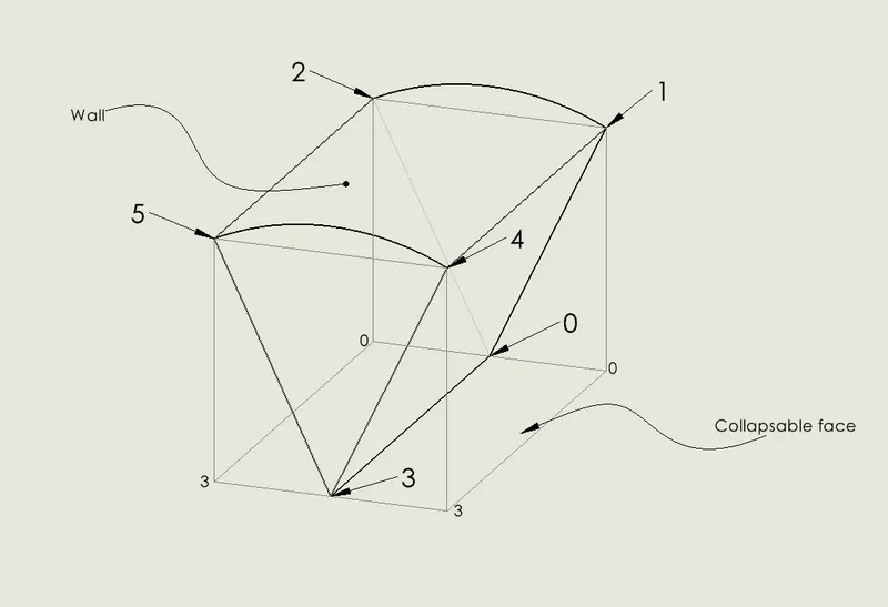
- The side faces of the sector/wedge have been asssigned 'symmetryPlane' condition since they are the symmetric planes. the benefit of doing so is to reduce the size of the mesh and the computational power required, since other regions on either side of these planes will have identical values.
- The block is numbered from back to front, with its `X-`axis being in the radial direction edge 0-1, `Y-`axis being along the arc 1--2, and edge 2-0 completing the plane. `Z-`axis is along edge 0 -3.
- A total of 4000 cells are being considered in the block.
- The wedge, which is actually a prism, has been initialised as a hexahedral using the collapsable face 0-3-3-0.
Input/Output control
Input and output controls are manipulated using the controlDict File of the simulation
/*--------------------------------*- C++ -*----------------------------------*
  =========                 |
  \      /  F ield         | OpenFOAM: The Open Source CFD Toolbox
   \    /   O peration     | Website:  https://openfoam.org
    \  /    A nd           | Version:  10
     \/     M anipulation  |
*---------------------------------------------------------------------------*/
FoamFile
{
    format      ascii;
    class       dictionary;
    location    "system";
    object      controlDict;
}
// * * * * * * * * * * * * * * * * * * * * * * * * * * * * * * * * * * * * * //

application     icoFoam;

startFrom       startTime;

startTime       0;

stopAt          endTime;

endTime         5;

deltaT          0.01;

writeControl    runTime;

writeInterval   0.1;

purgeWrite      0;

writeFormat     ascii;

writePrecision  6;

writeCompression off;

timeFormat      general;

timePrecision   6;

runTimeModifiable true;


// ************************************************************************* //
Boundary conditions for U :
Using the formula for `R_e`, the average inlet velocity of the flow is obtained by substituting the values for diameter and kinematic viscocity. Through hit and trial, it was observed that for this simulation, a kinematic viscocity of `1e-4` is suited for this mesh. The average inlet velocity comes out to be `2.1m//s`. The outlet velocity is set to zeroGradient condition, i.e. it is obtained using interpolation of values of nearby cells.
A noSlip condition is applied to the pipe wall in order to establish zero velocity at the wall.
/*--------------------------------*- C++ -*----------------------------------*
  =========                 |
  \      /  F ield         | OpenFOAM: The Open Source CFD Toolbox
   \    /   O peration     | Website:  https://openfoam.org
    \  /    A nd           | Version:  10
     \/     M anipulation  |
*---------------------------------------------------------------------------*/
FoamFile
{
    format      ascii;
    class       volVectorField;
    object      U;
}
// * * * * * * * * * * * * * * * * * * * * * * * * * * * * * * * * * * * * * //

dimensions      [0 1 -1 0 0 0 0];

internalField   uniform (0 0 2.10);

boundaryField
{
    inlet
    {
        type            fixedValue;
        value           uniform (0 0 2.10);
    }

    outlet
    {
        type            zeroGradient;
    }
    top
    {
        type            noSlip;
    }
    bottom
    {
        type            zeroGradient;
    }
    side1
    {
        type            symmetryPlane;
    }
    side2
    {
        type            symmetryPlane;
    }

}

// ************************************************************************* //
Boundary Conditions for P
The inlet pressure is set to zerogradient while the output pressure has been set to the fixed value of `0` . Our main aim with pressure is to verify wheather to pressure gradient obtained through Hagen Poiseuilli's equation is actually obtained in the solution.
/*--------------------------------*- C++ -*----------------------------------*
  =========                 |
  \      /  F ield         | OpenFOAM: The Open Source CFD Toolbox
   \    /   O peration     | Website:  https://openfoam.org
    \  /    A nd           | Version:  10
     \/     M anipulation  |
*---------------------------------------------------------------------------*/
FoamFile
{
    format      ascii;
    class       volScalarField;
    object      p;
}
// * * * * * * * * * * * * * * * * * * * * * * * * * * * * * * * * * * * * * //

dimensions      [0 2 -2 0 0 0 0];

internalField   uniform 0;

boundaryField
{
    inlet
    {
        type            zeroGradient;
    }

    outlet
    {
        type            fixedValue;
        value           uniform 0;
    }
    top
    {
        type            zeroGradient;
    }
    bottom
    {
        type            zeroGradient;
    }
    side1
    {
        type            symmetryPlane;
    }
    side2
    {
        type            symmetryPlane;
    }
}

// ************************************************************************* //
OBSERVATIONS -
Velocity Profile:
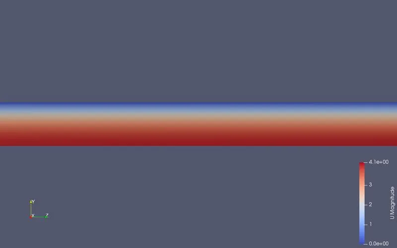
The velocity profile of the flow at different distances along the pipe's length is shown as follows. It is observed plainly that the velocity at the walls is nearly 0, while it progressively increases downwards, becoming maximum at the base.
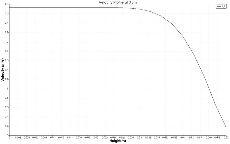
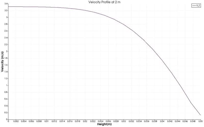
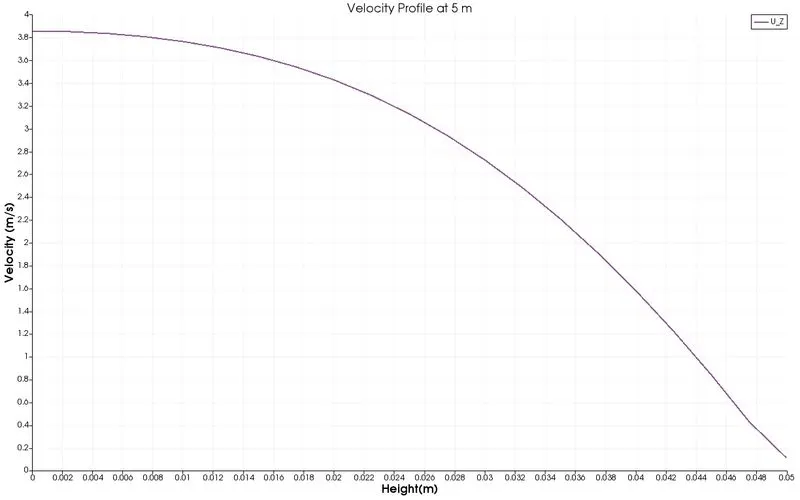
We can observe that the velocity profile plateaus at the top initially, but as the length progresses it becomes more parabolic.
Pressure distribution:
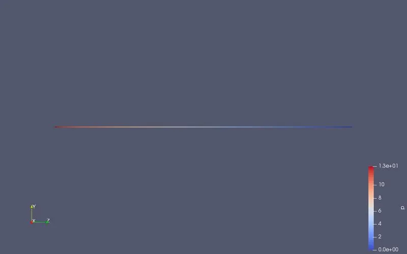
We can see the pressure gradient vividly across the pipe. Near the inlet, greater pressure is required to accelerate the flow and overcome friction. Once it becomes fully developed, pressure is only required to overcome friction.
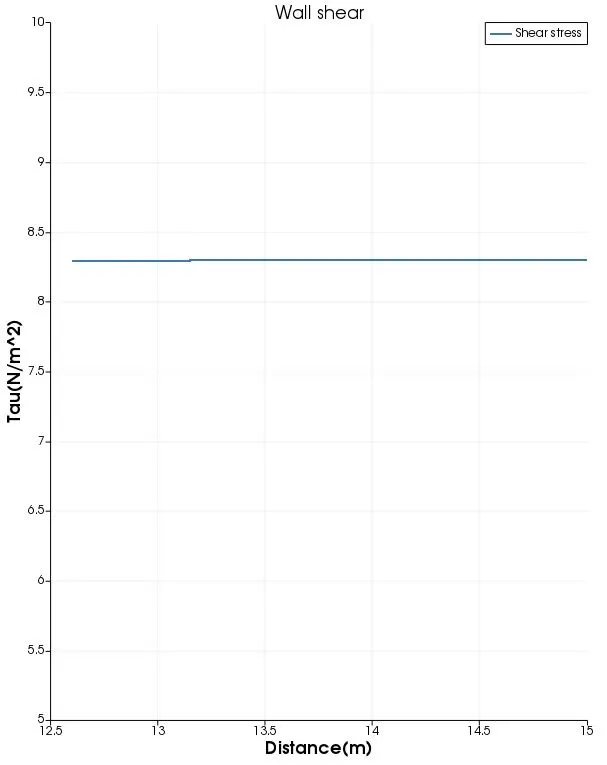
Wall shear: Wall shear stress acting on the fluid at different time steps are shown as follows
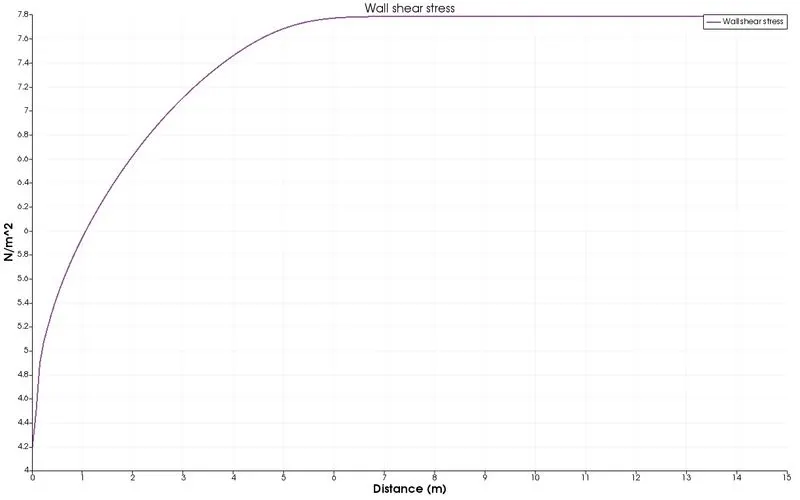
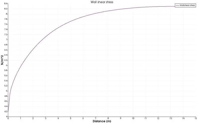
I Image 1 shows stress at time(t)=2.5s; Image 2 shows stress at time(t)=5s
The wall stress acting on the fluid after a time of 5 seconds is :
| S.No | Length(m) | Shear Stress(N/m^2) |
| 1 | 0 | 4.2 |
| 2 | 1.5 | 6.32014 |
| 3 | 3 | 7.11154 |
| 4 | 4.5 | 7.59726 |
| 5 | 6 | 7.89282 |
| 6 | 7.5 | 8.07358 |
| 7 | 9 | 8.18522 |
| 8 | 10.5 | 8.25379 |
| 9 | 12 | 8.28763 |
| 10 | 13.5 | 8.29581 |
| 11 | 15 | 8.29638 |
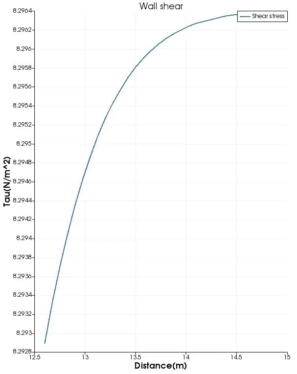
The shear stress distribition for fully developed flow
INFERENCE:
Velocity profiile:
As per the formula for entrance length, `L_e` for our simulation comes out to be `12.6m`. While the simulation also reflects this, the variation at different distances is too small since the length of the pipe is so long. Therefore we can conclude that even though the flow would be fully developed only afer 12.6m, the practical difference is negligable.
We also observe that the profile becomes progressively parabolic showing that the boundary layer finally converges at the centre
Pressure gradient:
The analytical pressure gradient comes out to be `1.6128Pa`. The simulated pessure gradient at a distance of `12.6m`from the origin is `1.62765Pa`. This is a `%`error of `0.92%`, which is within the permissible limit.
Shear stress:
It is observed that as the length increases, the shear stress also increases as the velocity does. However, for a fully developed flow, there is barely any variation in wall shear stress , showing that the central velocity remains constant and unchanged in that region of the pipe. To put the variation in values of the shear stress into perpective-