Week 7 - Simulation of a 1D Super-sonic nozzle flow simulation using Macormack Method
AIM: To study the flow in a quasi-1D supersonic nozzle using Macormack's method and comparing the observations obtained from using conservative and non conservative governing equations.
THEORY:
Nozzle :-
A nozzle is a device which increases the kinetic energy of a fluid at the cost of its pressure. It most daily life applications, the Mach number(M; ratio of speed of fluid in the medium at a point to the speed of sound in that medium at that point) is less than 1, thereby bringing about an increase in velocity through a decrease in area (resulting in convergent structure). However when M > 1, then an increase in velocity can be obtained only through an increase in area ( resulting in divergent structutre). This is the basis for supersonic flow.
`(dA)/A = (dV)/V(M^2 - 1)`; area velocity relation for compressive flow.
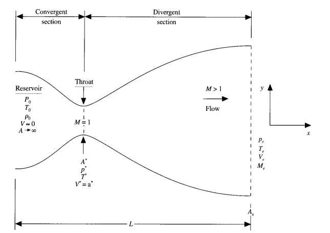
Fluid flow in a nozzle is not a true one dimensional flow because area of crossection changes as a function of x. Hence it is supposed to be a 2 dimensional flow, with properties varying along both x and y axis. However we assume that the properties are uniform across a cross section, thereby making the flow quasi 1 dimensional.
Governing equations:-
The three governing equations considered are those of continuity, momentum and energy conversation. These equations can be expressed in both conservative (fixed control volume) and non conservative (moving control volume) depending on the system being considered.
ρ = Density ; P = Pressure ; V = Velocity ; A = Area ; T = Temperature ; γ = specific heat ratio; Cv = Specific heat at constant volume; a = speed of sound in the reservoir; L = length of the nozzle
Non dimensionalising of the variables are also done, mainly in order to add an aesthetic advanatge in terms of data representation. It is done as follows:
x' = `x/L`; P' = `P/(Po)`; V' = `V/(Vo)`; t' = `t/(L/a)`; ρ' = `ρ/(ρo)`; T' = `T/(To)`
Equation of continuity-
`(∂(ρA))/(∂t) + (∂(ρAV))/(∂x) = 0`
- expanding the differential
`A(∂ρ)/(∂t) = -AV(∂ρ)/(∂x) - ρV(∂A)/(∂x) -ρA(∂V)/(∂x)`
- dividing by A
`(∂ρ)/(∂t) = -V(∂ρ)/(∂x) - (ρV)/A(∂A)/(∂x) -ρ(∂V)/(∂x)`
`(∂ρ)/(∂t) = -V(∂ρ)/(∂x) - ρV(∂lnA)/(∂x) -ρ(∂V)/(∂x)`
- In non dimensional form
`(∂ρ')/(∂t') = -V'(∂ρ')/(∂x') - ρ'V'(∂lnA')/(∂x') -ρ'(∂V')/(∂x')`
Equation of momentum conservation-
`ρ(∂V)/(∂t) + ρV(∂V)/(∂x) = -(∂P)/(∂x)`
- dividing by ρ
`(∂V)/(∂t) = -V(∂V)/(∂x) -1/ρ(∂P)/(∂x)`
- putting P = ρRT based on ideal gas equation
`(∂V)/(∂t) = -V(∂V)/(∂x) -R((∂T)/(∂x) - T/ρ(∂ρ)/(∂x))`
- In non dimensional form
`(∂V')/(∂t') = -V'(∂V')/(∂x') -(1/γ)((∂T')/(∂x') - T'/ρ'(∂ρ')/(∂x'))`
Equation of energy conservation-
`ρA(∂e)/(∂t) + ρAV(∂e)/(∂x) = -P(∂(AV))/(∂x)`
- dividing by ρA and putting e = CvT
`C_v(∂T)/(∂t) + C_vV(∂T)/(∂x) = -P/(ρA)(V(∂A)/(∂x)+ A(∂V)/(∂x))`
`C_v(∂T)/(∂t) + C_vV(∂T)/(∂x) = -P/ρ(V(∂lnA)/(∂x)+ (∂V)/(∂x))`
- dividing by Cv and equating P = ρRT
`(∂T)/(∂t) = - V(∂T)/(∂x) -(RT)/(C_v)(V(∂lnA)/(∂x)+ (∂V)/(∂x))`
- since R/Cv = γ-1
`(∂T)/(∂t) = - V(∂T)/(∂x) -(γ-1)T(V(∂lnA)/(∂x)+ (∂V)/(∂x))`
- In non dimensional form
`(∂T')/(∂t') = - V'(∂T')/(∂x') -(γ-1)T'(V'(∂lnA')/(∂x')+ (∂V')/(∂x'))`
Code for non conservative flow:
close all
clear
clc
dx = 0.1;
x = 0:dx:3;
% initial conditions
rho = 1 - 0.3146 * x;
T = 1 - 0.2314 * x;
V = (0.1 + 1.09 * x).*(T.^0.5);
A = 1 + 2.2*(x - 1.5).^2;
P = rho.*T; % non dimensional pressure obtained from real gas equation

% time step
C = 0.35; % steady state ontained at around t = 800
% Time marching pre requisites
V_o = V;rho_o = rho;T_o = T;
drdt = zeros(size(x));
drdt_p = drdt; drdt_c = drdt; %initialising predictor and corrector values for all nodes
dvdt = zeros(size(V));
dvdt_p = dvdt; dvdt_c = dvdt;
dTdt = zeros(size(T));
dTdt_p = dTdt; dTdt_c = dTdt;
n = length(x);
n1 = 0;
%while err > 1e-4

for t = 1:900
    %n1 = n1 +1;
    V_o = V;rho_o = rho;T_o = T; % updating the old values with the new ones
    a = (T).^0.5; % non dimensional speed of sound in the medium
    dt = C*dx./(a+V); % time step calculation
    dt = min(dt); % taking uniform time step as the minimum time step

    for i = 2:length(x)-1 %loop for predictor step
        dvdx_p(i) = (V_o(i+1)-V_o(i))/dx;dAdx_p(i) = (log(A(i+1))-log(A(i)))/dx;drdx_p(i) = (rho_o(i+1)-rho_o(i))/dx;
        dtdx_p(i) = (T_o(i+1)-T_o(i))/dx;

        drdt_p(i) =  -(rho_o(i) * dvdx_p(i)) - (rho_o(i) * V_o(i) * dAdx_p(i)) - (V_o(i) * drdx_p(i));
        rho(i) = rho_o(i) + drdt_p(i) * dt;
        dvdt_p(i) = -(V_o(i) * dvdx_p(i)) -(1/1.4) * (dtdx_p(i) + (T_o(i)/rho_o(i)) * drdx_p(i));
        V(i) = V(i) + dvdt_p(i)* dt;
        dTdt_p(i) = -(V_o(i) * dtdx_p(i)) -(1.4 - 1) * T_o(i) * (dvdx_p(i) + V_o(i) * dAdx_p(i));
        T(i) = T_o(i) + dTdt(i) * dt;
    end

    for i = 2:length(x) - 1 % loop for corrector step
        dvdx_c(i) = (V(i)-V(i-1))/dx; dAdx_c(i) = (log(A(i))-log(A(i-1)))/dx; drdx_c(i) = (rho(i)-rho(i-1))/dx;
        dtdx_c(i) = (T(i)-T(i-1))/dx;

        drdt_c(i) =  -(rho(i) * dvdx_c(i)) - (rho(i) * V(i) * dAdx_c(i)) - (V(i) * drdx_c(i));
        dvdt_c(i) = -(V(i) * dvdx_c(i)) -(1/1.4) * (dtdx_c(i) + (T(i)/rho(i)) * drdx_c(i));
        dTdt_c(i) = -(V(i) * dtdx_c(i)) -(1.4 - 1) * T(i) * (dvdx_c(i) + V(i) * dAdx_c(i));
    end

    drdt = 0.5 * (drdt_p + drdt_c);
    dvdt = 0.5 * (dvdt_p + dvdt_c);
    dTdt = 0.5 * (dTdt_p + dTdt_c);

    for i = 2:length(x)-1 %loop for finally updating flow variables
        rho(i) = rho_o(i) + drdt(i) * dt;
        V(i) = V_o(i) + dvdt(i) * dt;
        T(i) = T_o(i) + dTdt(i) * dt;
        P(i) = rho(i) * T (i); % non dimensional pressure obtained from real gas equation
    end
    % inlet boundary conditions
    V(1) = 2*V(2) - V(3);
    % outlet boundary conditions
    V(n) = 2*V(n-1) - V(n-2);
    rho(n) = 2*rho(n-1) - rho(n-2);
    T(n) = 2*T(n-1) - T(n-2);


   subplot(4,1,1)
   plot(x,V,'Marker','o')
   title(sprintf('Time %d',t))
   ylabel("Velocity");xlabel("Distance");
   pause(0.00001)
   subplot(4,1,2)
   plot(x,T,'Marker','o')
   title(sprintf('Time %d',t))
   ylabel("Temperature");xlabel("Distance");
   subplot(4,1,3)
   plot(x,rho,'Marker','o')
   title(sprintf('Time %d',t))
   ylabel("Density");xlabel("Distance");
   subplot(4,1,4)
   plot(x,P,'Marker','o')
   title(sprintf('Time %d',t))
   ylabel("Pressure");xlabel("Distance");

end
Conseravtive form:
Equation of continuity-
`(∂(ρA))/(∂t) + (∂(ρAV))/(∂x) = 0`
- In non dimensional form
`(∂(ρ'A'))/(∂t') + (∂(ρ'A'V'))/(∂x') = 0`
Equation of momentum conservation-
`(∂(ρAV))/(∂t) + (∂(ρAV^2))/(∂x) = -A(∂P)/(∂x)`
- using `(∂(PA))/(∂x) - P(∂A)/(∂x)= A(∂P)/(∂x)`
`(∂(ρAV))/(∂t) + (∂(ρAV^2) + ∂(PA))/(∂x) = P(∂A)/(∂x)`
- In non dimensional form
`(∂(ρ'A'V'))/(∂t') + (∂(ρ'A'V' ^ 2) + 1/γ∂(P'A'))/(∂x') = 1/γP'(∂A')/(∂x')`
Equation for energy conservation
`(∂(ρ(e+V^2/2)A))/(∂t) + (∂(ρ(e+V^2/2)AV+PAV))/(∂x) =0`
- In non dimensional form
`(∂(ρ'((e' )/(γ-1)+γ/2V'^2))A')/(∂t') + (∂(ρ'((e')/(γ-1)+γ/2V'^2)A'V'+P'A'V'))/(∂x') =0`
In terms of dependent variables,U1,U2,U3, the above equations can be written as
`(∂U_1)/(∂t) = -(∂F_1)/(∂x)`
`(∂U_2)/(∂t) = -(∂F_2)/(∂x) +J_2`
`(∂U_3)/(∂t) = -(∂F_3)/(∂x)`
where
`F1 = U2`
`F2 = (U_2^2)/U_1+((γ-1)/γ)*(U_3-γ/2*U_2^2/U_1)`
`F3 = γ(U_3 * U_2)/U_1+(γ(γ-1))/2 * U_2^3 / U_1^2`
close all
clear
clc

dx = 0.1;
x = 0:dx:3; n = length(x);
A = 1 + 2.2*(x - 1.5).^2;
C = 0.5;

%initial conditions
rho = zeros(size(x)); T = zeros(size(x)); V = zeros(size(x));

for i=1:length(x)
    if x(i)>=0 && x(i)<0.5
        rho(i) = 1;
        T(i) = 1;
    elseif x(i)>=0.5 && x(i)<1.5
        rho(i) = 1 - 0.366*(x(i)-0.5);
        T(i) = 1 - 0.167*(x(i)-0.5);
    elseif x(i)>=1.5 && x(i)<=3
        rho(i) = 0.634 - 0.3879*(x(i)-1.5);
        T(i) = 0.833 - 0.3507*(x(i)-1.5);
    end
    V(i) = 0.59/(rho(i)*A(i));
end

% rho = 1 - 0.3146 * x;
% T = 1 - 0.2314 * x;
% V = (0.1 + 1.09 * x).*(T.^0.5);
% V = 0.59./(rho.*A);
% P = rho.*T;


%dependent variables
U1 = rho.*A;
U2 = (rho.*A).*V;
U3 = rho.*(T/(1.4-1)+(1.4/2) * V.^2).*A;
du1dt = zeros(size(x)); du2dt = zeros(size(x)); du3dt = zeros(size(x));
du1dt_p = zeros(size(x)); du2dt_p = zeros(size(x)); du3dt_p = zeros(size(x));
du1dt_c = zeros(size(x)); du2dt_c = zeros(size(x)); du3dt_c = zeros(size(x));


for t = 1:950
    U1_o = U1; U2_o = U2; U3_o = U3;
    F1 = U2;
    F2 = (U2.^2)./U1+((1.4-1)/1.4)*(U3 - (1.4/2)*(U2.^2)./U1);
    F3 = 1.4*(U3 .* U2)./U1 - (1.4*0.4)/2 * (U2.^3) ./ (U1.^2);
    J2 = (1/1.4) * rho .* T;

    %time step calculation
    a = T.^0.5;
    dt = C * dx./(a+V);
    dt = min(dt);

    for i = 2:length(x)-1
        df1dx_p(i) = (F1(i+1) - F1(i))/dx; df2dx_p(i) = (F2(i+1) - F2(i))/dx; df3dx_p(i) = (F3(i+1) - F3(i))/dx;
        dj2dx_p(i) = J2(i) * (A(i+1)-A(i))/dx;

        du1dt_p(i) = -df1dx_p(i); du2dt_p(i) = -df2dx_p(i) + dj2dx_p(i); du3dt_p(i) = -df3dx_p(i);
        U1(i) = U1_o(i) + du1dt_p(i)*dt;
        U2(i) = U2_o(i) + du2dt_p(i)*dt;
        U3(i) = U3_o(i) + du3dt_p(i)*dt;
    end

    V = U2./U1;
    rho = U1./A;
    T = 0.4 * (U3./U1 - 1.4/2 * V.^2);
    P = rho .* T;

    %updating boundary conditions before corrector step
    U1(1) = rho(1)*A(1);
    U2(1) = 2*U2(2) - U2(3);
    U3(1) = rho(1)*(T(1)/(1.4-1)+1.4/2 * V(1)^2)*A(1);

    U1(n) = 2*U1(n-1) - U1(n-2);
    U2(n) = 2*U2(n-1) - U2(n-2);
    U3(n) = 2*U3(n-1) - U3(n-2);

    F1 = U2;
    F2 = (U2.^2)./U1+((1.4-1)/1.4)*(U3-(1.4/2)*(U2.^2)./U1);
    F3 = 1.4*(U3 .* U2)./U1 - ((1.4*0.4)/2) * (U2.^3) ./ (U1.^2);
    J2 = (rho.*T)/1.4;

    for i = 2:length(x)-1
        df1dx_c(i) = (F1(i) - F1(i-1))/dx; df2dx_c(i) = (F2(i) - F2(i-1))/dx; df3dx_c(i) = (F3(i) - F3(i-1))/dx;
        dj2dx_c(i) = J2(i) * (A(i)-A(i-1))/dx;

        du1dt_c(i) = -df1dx_c(i); du2dt_c(i) = -df2dx_c(i) + dj2dx_c(i); du3dt_c(i) = -df3dx_c(i);
    end

    du1dt = 0.5*(du1dt_p+du1dt_c);
    du2dt = 0.5*(du2dt_p+du2dt_c);
    du3dt = 0.5*(du3dt_p+du3dt_c);

    for i = 2:length(x)-1
        U1(i) = U1_o(i) + du1dt(i)*dt;
        U2(i) = U2_o(i) + du2dt(i)*dt;
        U3(i) = U3_o(i) + du3dt(i)*dt;
    end

    U1(1) = rho(1)*A(1);
    U2(1) = 2*U2(2) - U2(3);
    U3(1) = rho(1)*(T(1)/(1.4-1)+1.4/2 * V(1)^2)*A(1);

    U1(n) = 2*U1(n-1) - U1(n-2);
    U2(n) = 2*U2(n-1) - U2(n-2);
    U3(n) = 2*U3(n-1) - U3(n-2);

    V = U2./U1;
    rho = U1./A;
    T = 0.4 * (U3./U1 - 1.4/2 * V.^2);
    P = rho .* T;
    mfr = mfr_co(rho,A,V); %mass flow rate

    subplot(4,1,1)
    plot(x,V,'Marker','o')
    title(sprintf('Time %d',t))
    ylabel("Velocity");xlabel("Distance");
    pause(0.00001)
    subplot(4,1,2)
    plot(x,T,'Marker','o')
    title(sprintf('Time %d',t))
    ylabel("Temperature");xlabel("Distance");
    subplot(4,1,3)
    plot(x,rho,'Marker','o')
    title(sprintf('Time %d',t))
    ylabel("Density");xlabel("Distance");
    subplot(4,1,4)
    plot(x,P,'Marker','o')
    title(sprintf('Time %d',t))
    ylabel("Pressure");xlabel("Distance");

    plot(x,mfr,'Marker','o')
    title(sprintf('Time %d',t))
    ylabel("Pressure");xlabel("Distance");


end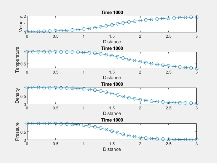
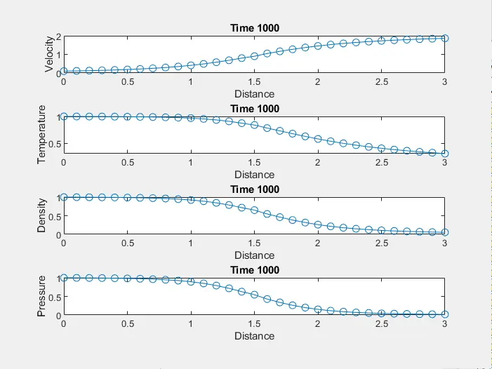
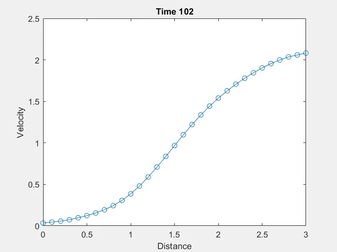
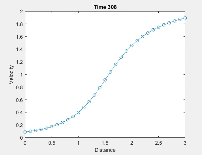
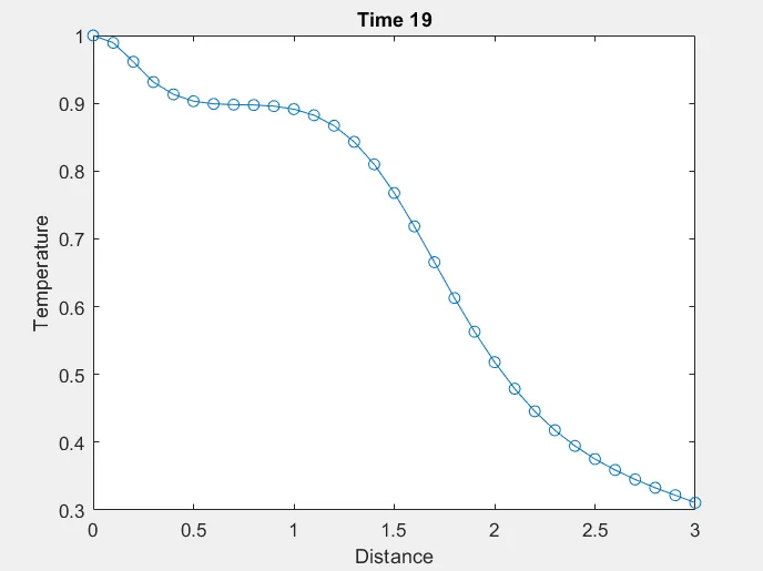
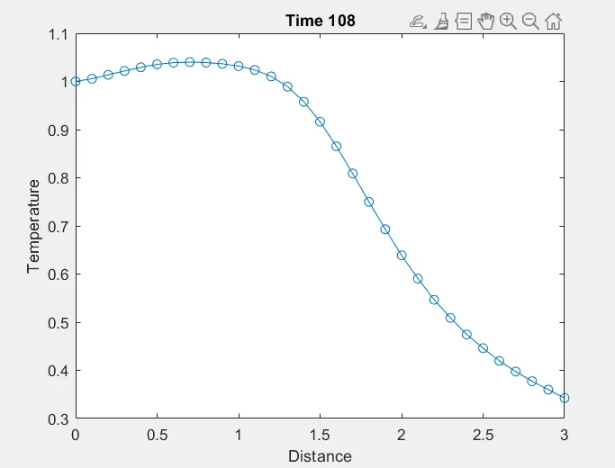
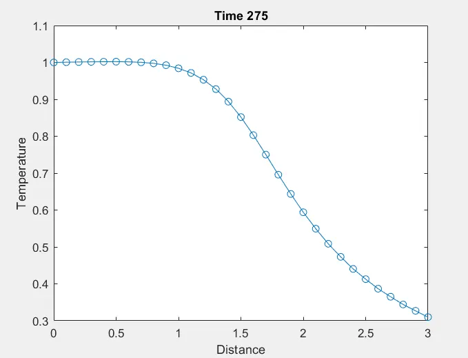
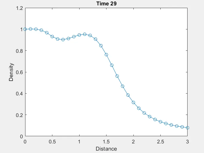
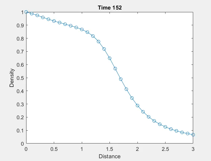
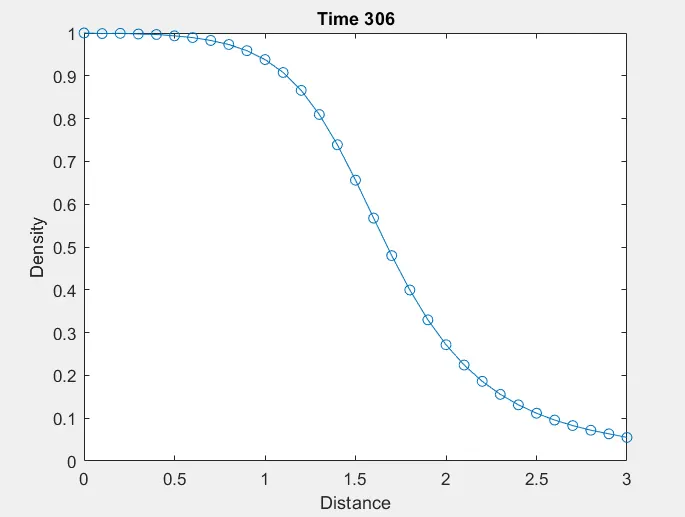
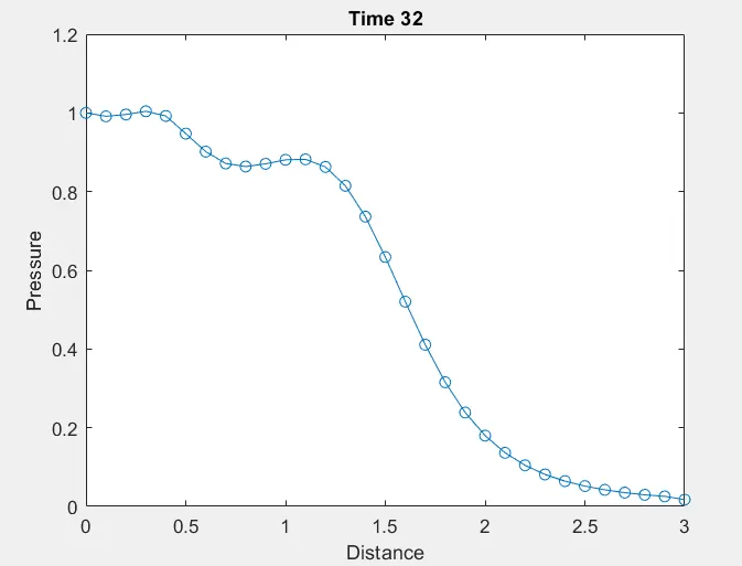
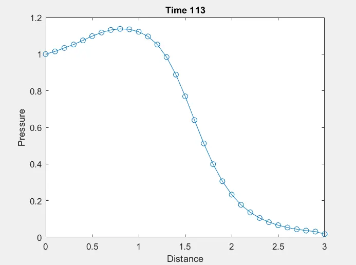
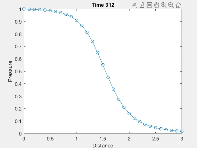
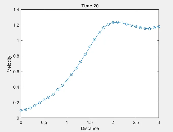
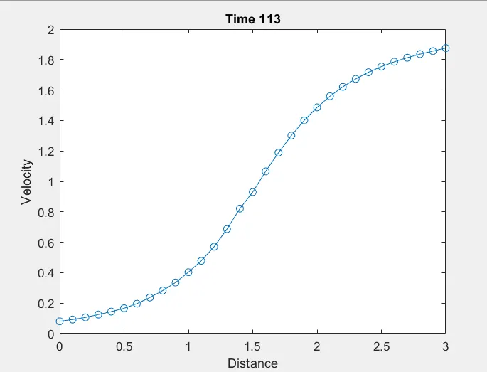
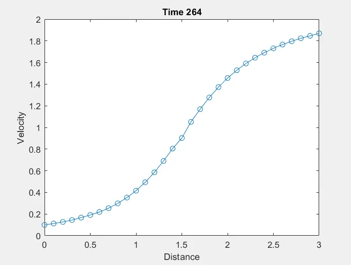
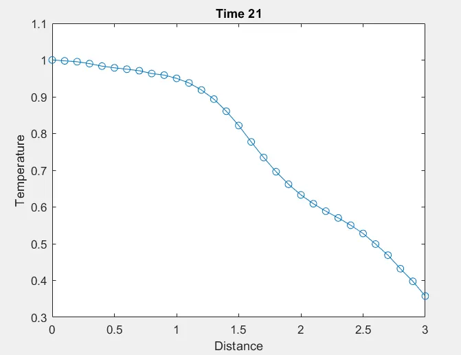
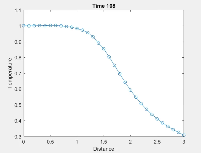
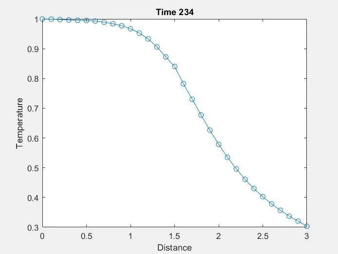
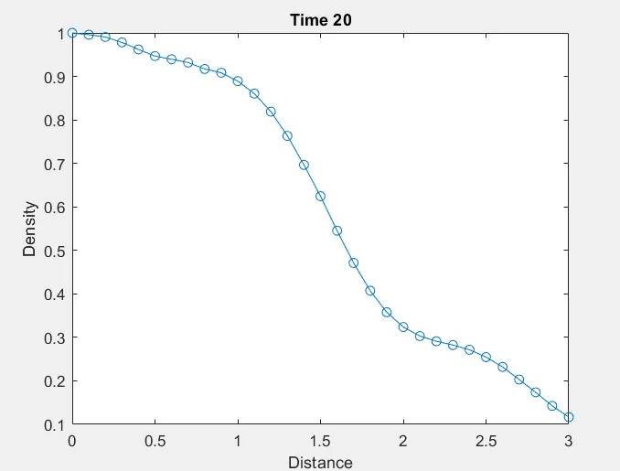
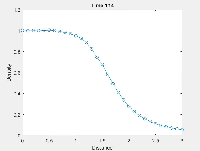
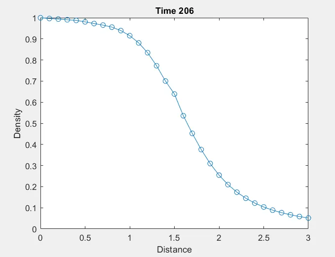
Time wise distribution of primtive variables under conservative governing equations
Velocity
Temperature
Density
Pressure
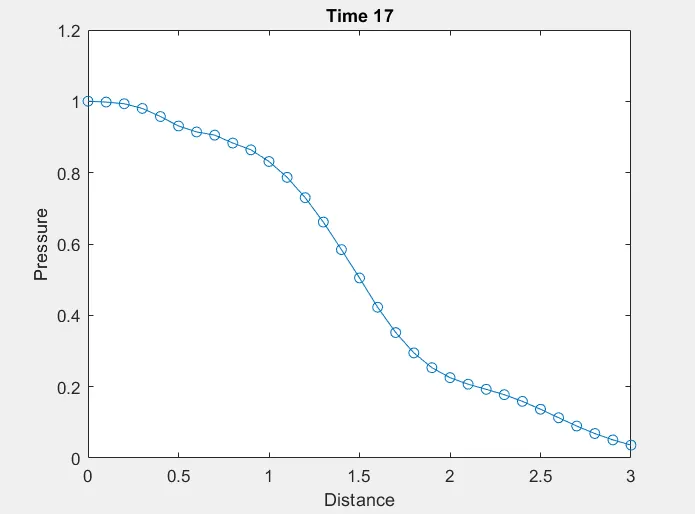
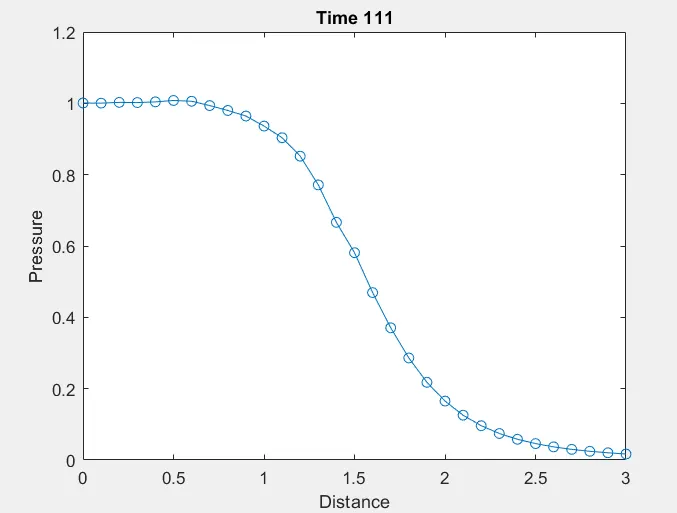
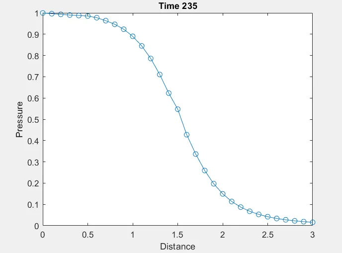
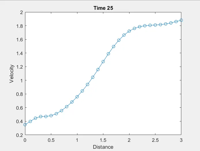
It is evidently seen that the conservative form reaches a steady state at around 200 time steps in comparison to the non conservative form which stabalises around 300 time steps
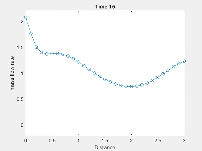
3) Mass flow rate of at different time steps
Non conservative form:
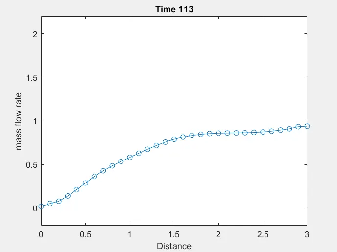
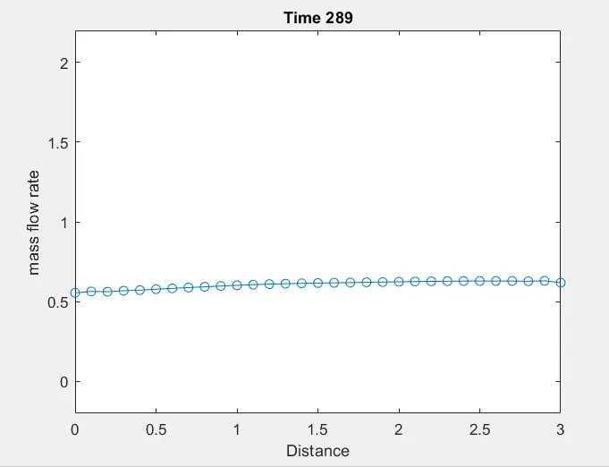
Conservative form:
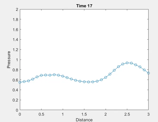
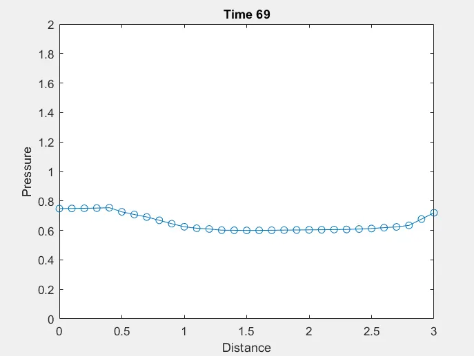
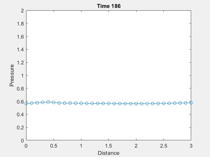
While the end result is same in both the forms, The mass flow rate remains more consistent in the conservative form as compared to the non conservative form.
4) Comparison of Normalised mass flow rate
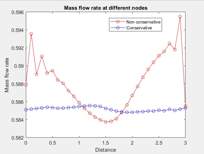
There are small variations in the mass flow rate in between nodes in the non conservative form while it is nearly uniform in the conservative.
5) Mach number distribution from subsonic to supersonic state
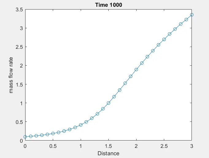
Inference:
While result wise, both non conservative and conservative form yields the same result, the Non conservative form is more susceptable to shocks. The conservative form provides a more stable result on the other hand.
Grid independence test
Velocity at index at which x = 1.5
In the non conservative form:
for dx = 0.1 V = 0.91 ; dx = 0.01 V = 0.96, dx = 0.001 V = 1.36
Here the % increase is greater than 5%
In the conservative form:
for dx = 0.1 V = 0.9 ; dx = 0.01 V = 0.93, dx = 0.001 V = 1.89
Here the percentage change is less than 4%, thus making it much more acceptable.
Inference: Largely both the models are grid independent, but the conservative model shows greater levels ofgrid independence.
Design of code:
The variables used have been explained in the theory
Most other explanations have been given alongside inn the form of comments
Mass flow rate has been obtained using the functions
function mfr = mfr_co(rho,A,V)
% A function which accepts the density, area and velocity of flow
% in order to calculate the mass flow rate
mfr = (rho.*A).*V;
end
function mfr = mfr_nonco(rho,A,V)
% A function which accepts the density, area and velocity of flow
% in order to calculate the mass flow rate
mfr = (rho.*A).*V;
end