Week 8 - Simulating Cyclone separator with Discrete Phase Modelling
Simulating Cyclone separator with Discrete Phase Modelling
Aim: To perform analysis on cyclone separator and calculate the separation efficiency and pressure drop.
Objective:
- To write a few words about any four empirical models used to calculate the cyclone separator efficiency.
- To perform an analysis on a given cyclone separator model by varying the particle diameter from 1 μm to 5 μm and calculate the separation efficiency in each case. Discuss the results. [Use both the velocity's as 3m/sec.]
- To perform an analysis on a given cyclone separator model by varying the particle velocity from 1 m/sec to 5 m/sec and calculate the separation efficiency and pressure drop in each case. Discuss the results. [Use particle diameter size as 5 μm for all cases & keep flow velocity same as particle velocity]
Introduction:
A cyclone separator is also called a cyclonic dust collector, which is a widely used as air pollution control device that cleans flue gases of particulate matter before such gases exit into the atmosphere. It's a method of collecting up to 99% of airborne waste in an easy-to-empty container beneath the cyclone.
These devices are primarily labeled as pre-cleaners, as they are instrumental in removing large and abrasive particles from flue gases, which then go through additional filtration processes to remove fine particulate matter. The relevance of cyclone separators lies in the fact that they facilitate the first step of the flue gas filtration process. The objective of these devices is to minimize air pollution and environmental hazards caused by production plant exhaust.
Cyclone separators work as a buffer against damage to enhanced filtration systems that can be adversely impacted by large and abrasive particulate matter. This, in turn, can negate the pollution control process applicable to flue gases emanating from production plants.
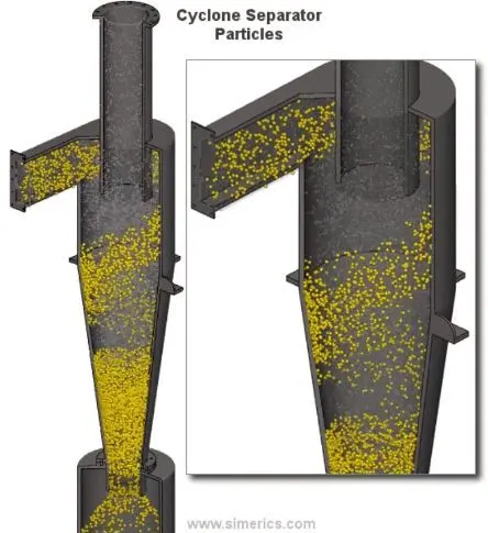
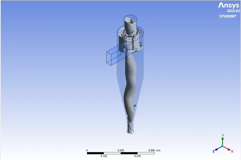
Cyclone separators work much like a centrifuge, but with a continuous feed of dirty air. In a cyclone separator, dirty flue gas is fed into a chamber. The inside of the chamber creates a spiral vortex, similar to a tornado. This spiral formation and the separation is shown in Figure . The lighter components of this gas have less inertia, so it is easier for them to be influenced by the vortex and travel up it. Contrarily, larger components of particulate matter have more inertia and are not as easily influenced by the vortex.
- Iozia and Leith model:
Iozia and leith logistic model is a modified version of Barth model, which is developed based on force balance. The model assumes that a particle carried by the vortex endures the influence of two forces that are centrifugal force Z and a flow resistance W. The collection efficiency of particle diameter dpi can be calculated from
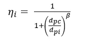
β is an expression for slope diameter
- Li & Wang model:
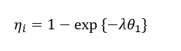
The Li and wang model includes particle bouncing or entrainment and turbulent diffusion at cyclone wall. A two-dimensional analytical expression of particle distribution in the cyclone is obtained.
Assumptions were made in making the model:
The radial particle velocity and the radial concentration profile are not constant for uncollected particles within the cyclone.
Boundary conditions with the consideration of turbulent diffusion coefficient and particle bounce re- entrainment on the cyclone wall are:
The collection efficiency of particle of any size is given as:
- Koch and litch model:
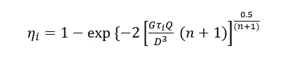
kotch and litch collection theory recognized the inherently turbulent nature of cyclones and the distribution of gas residence times within the cyclone. kotch and litch described the particle motion in the entry and collection regions with additional following assumptions:
The tangential velocity of a particle is equal to the tan- gential velocity of the gas flow, i.e. there is no slip in the tangential direction between the particle and the gas.
The tangential velocity is related to the radius of cyclone by: uR^n= constant.
- Lapple model:
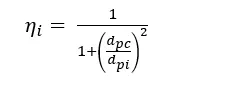
Lapple model was developed based on force balance without considering the flow resistance. Lapple assumed that a particle entering the cyclone is evenly distributed across the inlet opening. The particle that travels from inlet half width to the wall in the cyclone is collected with 50% efficiency. The semi empirical relationship developed by Lapple to calculate a 50% cut diameter.
Procedure/ steps to simulation of cyclone separator:
1. Geometry Creation:
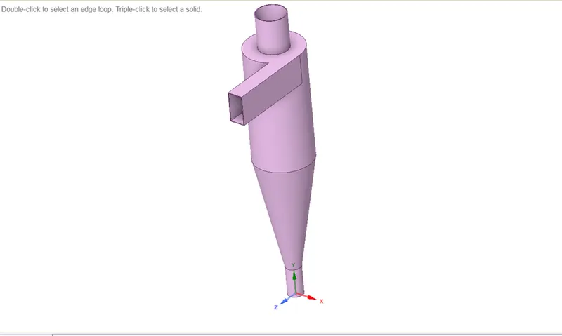
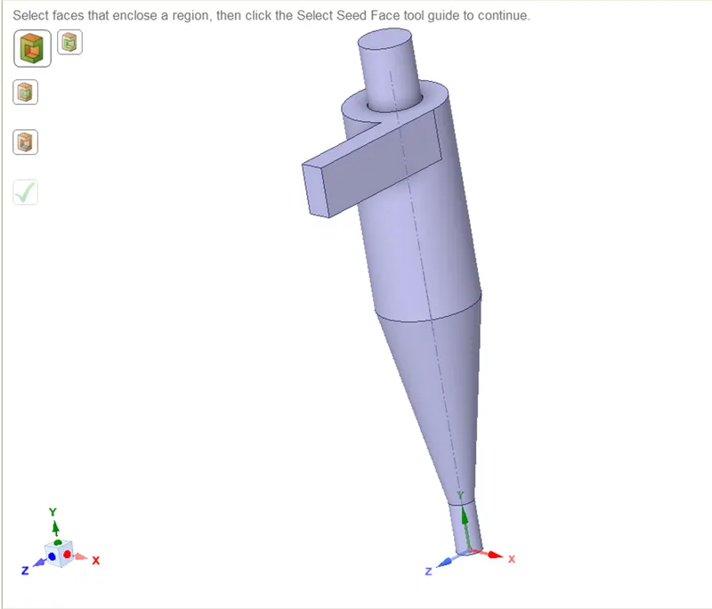
Importing the 3D geometry into spaceclaim, then extract the volume model from solid model by the help of volume extraction by 1 inlet and 2 outlet ports. Move the extracted part to meshing section.
Solid model of cyclone separator:
Extracted volume of cyclone separator:
2. Mesh:
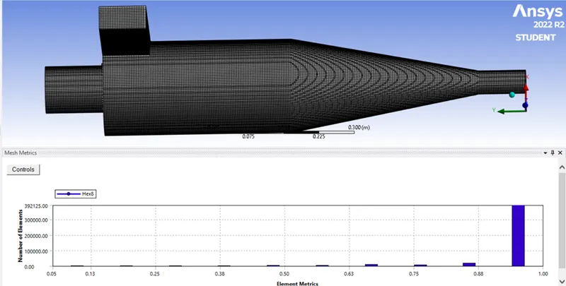
Allowing the cyclone separator geometry into meshing section, for case1 and case2 we use the different mesh sizes and types. In mean that for case1 we use the mesh method as Cartesian mesh with mesh size of 0.005m. From this mesh we get the Elements of 427871 and Nodes of 456604. The bellowed images show the 0.005m mesh size with cartesian cutcell mesh method.
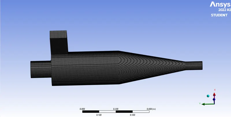
Element quality of cyclone separator:
Setup:
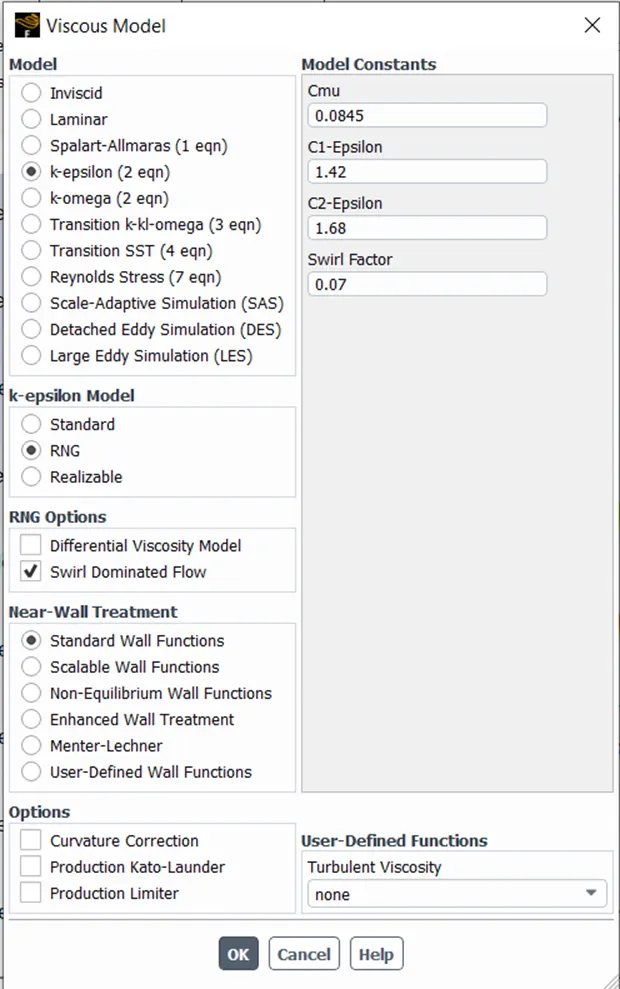
After meshing we have to setup the operation to perform the simulation. While entering into setup section we have to check the mesh, then enable the pressure based solver with steady state and gravitational acceleration as -9.81 ( negative gravity) in y-direction. After solver setup select the viscous model as in image that for enhanced accuracy of RNG model with k-espilon with swirl dominated flow and standard wall function treatment to be considered.
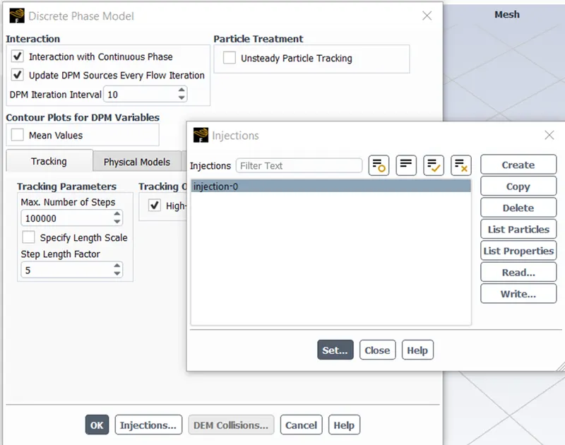
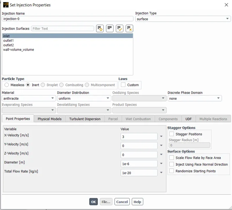
We have to simulate this simulation with discrete phase model (DPM). Enabling the Iteration with continuous phase and update DPM sources every flow Iteration. Giving the number steps as 100000. After than creating the injection with surface injection type at inlet of the geometry.
For anthracite material we allow the parameter, for velocity allow 3m/s and for diameter of particles we allow the 1micron to 5micron with constant flow rate of 1e-20.
Setting the boundary condition for cyclone separator as
Inlet velocity: 3m/s (constant) with DPM as reflect condition.
Outlet 1 (top): 0 Pa with DPM as escape condition.
Outlet 2 (bottom): 0 Pa with DPM as trap condition.
Initializing the simulation with standard initialization that compute from inlet of cyclone separator. Before this we have to enable the solution method as simple with turbulent kinetic energy and turbulent dissipation rate as second order upwind.
Performing the simulation with particle diameter as 1micro meter:
Residual plot:
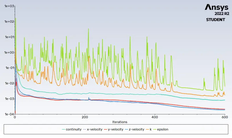
Separation efficiency = No. of Particle trapped/No. of Particle tracked
Then we got the efficiency as separation eff. = 325/378
Separation efficiency at 1m/s = 85.97%
Then export the particle data to post-process/result section to simulate and find out the flow of particle in cyclone separator and to simulate the problem with animation.
Post-process:
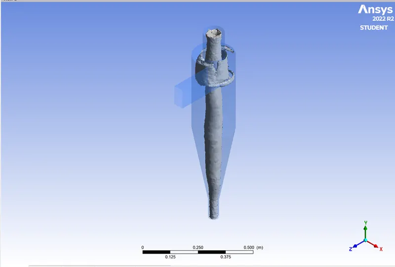
Import the particle data and enable the tracked particle move from cyclone separator, observe the particle exit at outlet (bottom) and outlet (top). Create the animation which provides the video of movement of particles in cyclone separator.
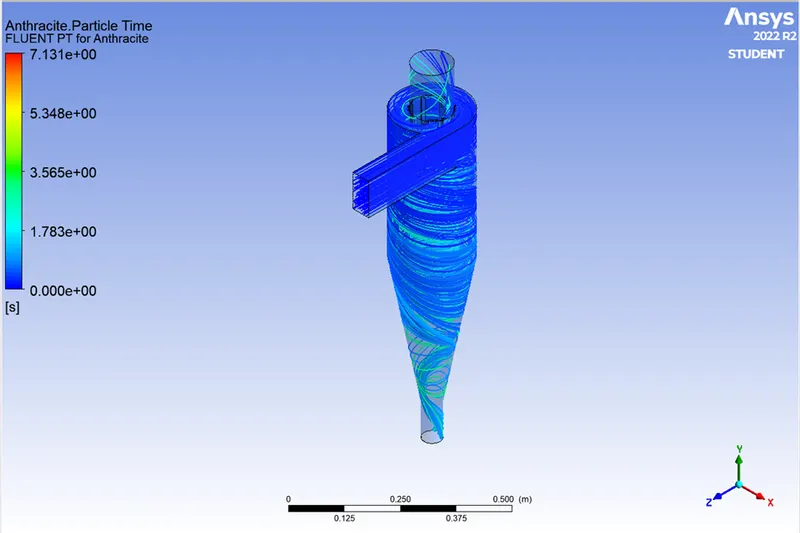
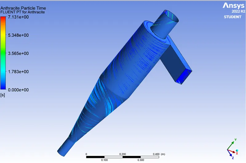
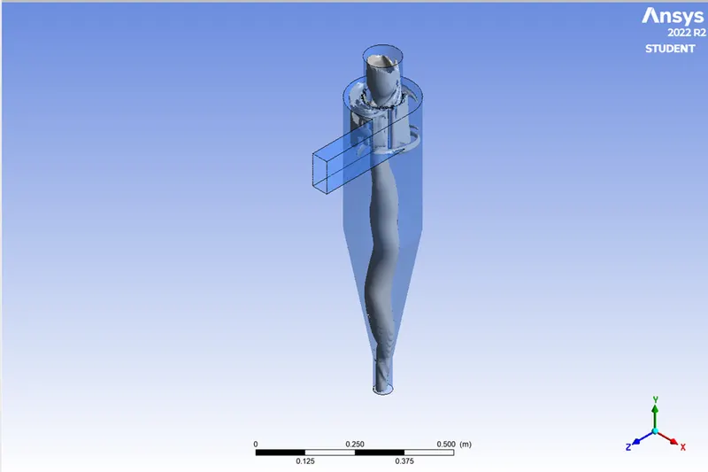
https://drive.google.com/file/d/1HWlqtuLnmhlpLIn4iZKAtkR2_vubxq9c/view?usp=share_link
Performing the simulation with particle diameter as 2micro meter:
Residual plot:
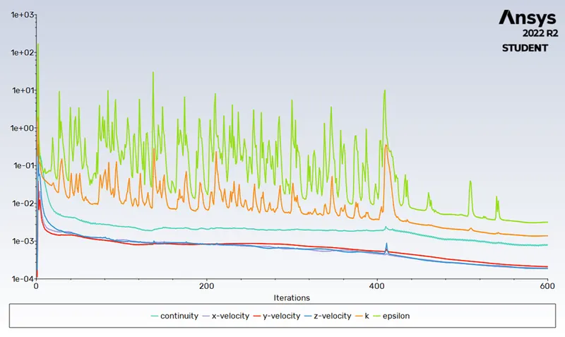
Separation efficiency = No. of Particle trapped/No. of Particle tracked
Then we got the efficiency as separation eff. = 331/378
Separation efficiency at 1m/s = 87.56%
Post-Process:
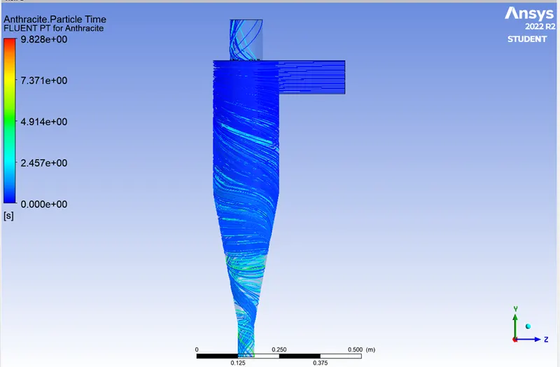
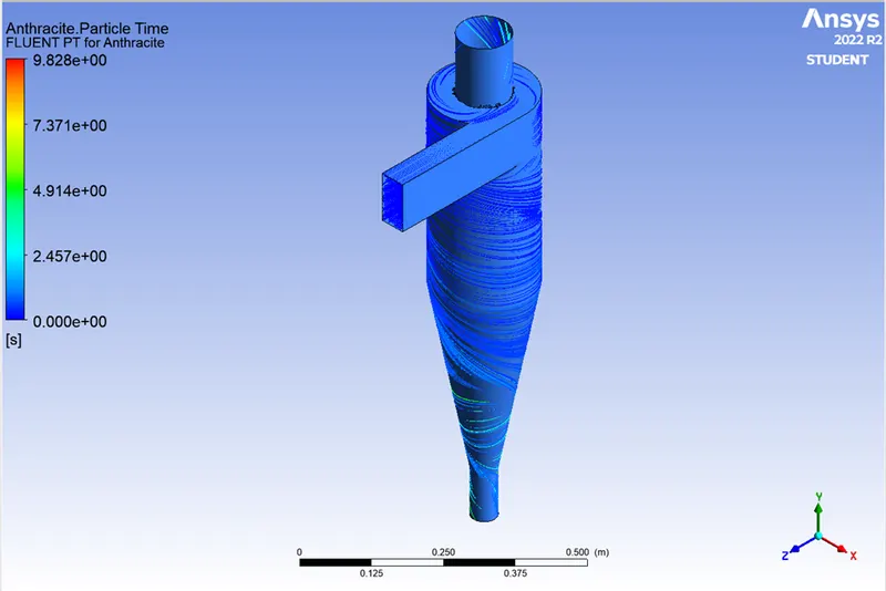
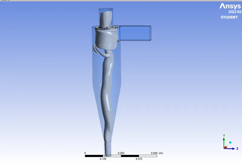
https://drive.google.com/file/d/1-4cMLnWg9qx3g0mKAPnnn7ylkLP-U9bg/view?usp=share_link
Performing the simulation with particle diameter as 3micro meter:
Residual plot:
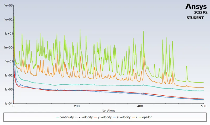
Separation efficiency = No. of Particle trapped/No. of Particle tracked
Then we got the efficiency as separation eff. = 336/378
Separation efficiency at 1m/s = 88.88%
Post-Process:
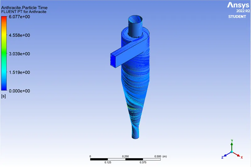
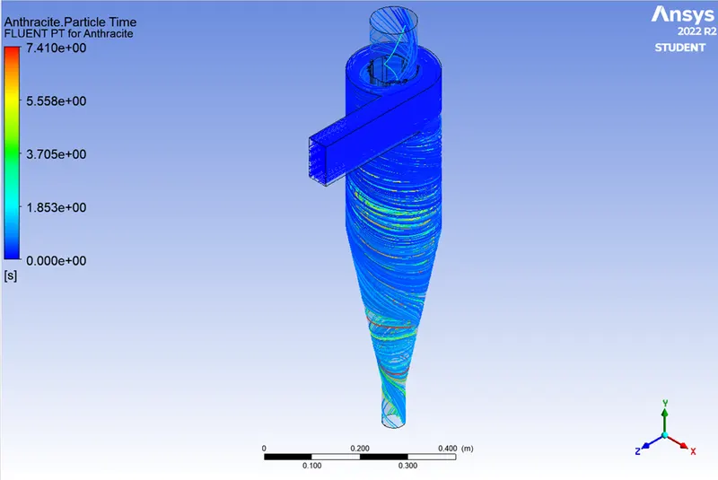
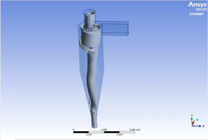
https://drive.google.com/file/d/1JWDSNF5C_8FDQMtZpRtkEvcZAkQz2zjg/view?usp=share_link
Performing the simulation with particle diameter as 4micro meter:
Residual plot:
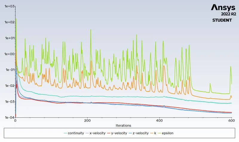
Separation efficiency = No. of Particle trapped/No. of Particle tracked
Then we got the efficiency as separation eff. = 351/378
Separation efficiency at 1m/s = 92.85%
Post-Process:
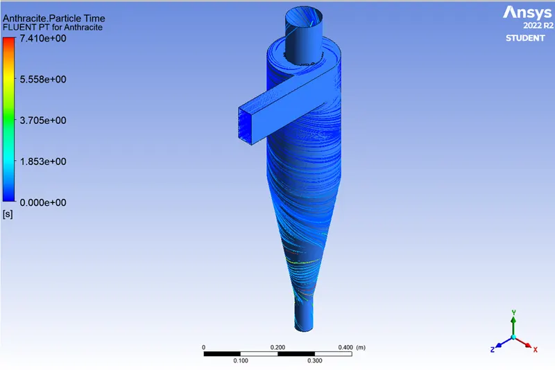
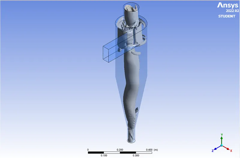
https://drive.google.com/file/d/1vlQuIUmKb6E-In6EBZPVelVaJqmkcSWS/view?usp=share_link
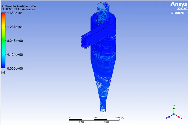
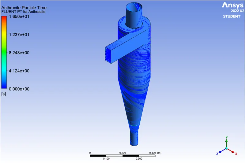
Performing the simulation with particle diameter as 5micro meter:
Residual plot:
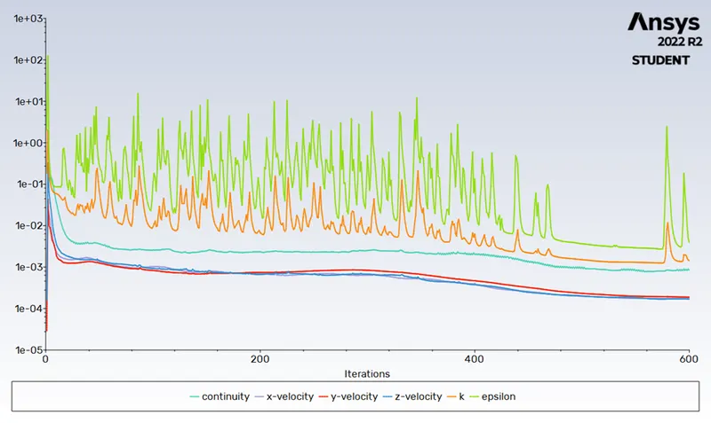
Separation efficiency = No. of Particle trapped/No. of Particle tracked
Then we got the efficiency as separation eff. = 377/378
Separation efficiency at 1m/s = 99.7%
Post-Process:
https://drive.google.com/file/d/1Im66-RoiYm4Rhabl-F5Qdjf6a9HR--3p/view?usp=share_link
CASE 2:
Mesh:
Allowing the cyclone separator geometry into meshing section, and refining the mesh size with named selection of 1 inlet and 2 inlet.
In this section we get the statistics as 377294 elements and 73741 nodes.
Setup:
Here we will consider same setup of case1 of solver, Discrete phase model (DPM) with changing some parameters of velocity as 1m/s to 5m/s with constant maintain of particle diameter of 5micron meter and keeping the inlet velocity same as particle velocity parameter. Other than setup will be same as case1 setup.
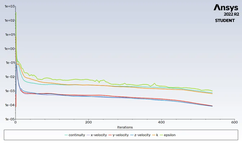
Performing the simulation with particle diameter as 5micro meter at velocity of 1m/s:
Residual plot:
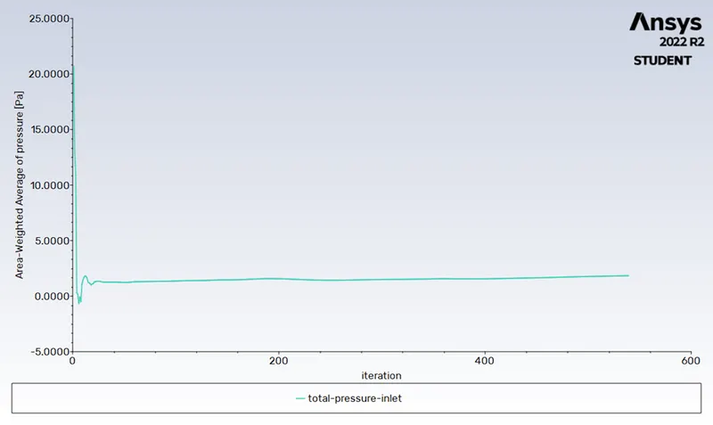
Pressure inlet:
Outlet pressure:
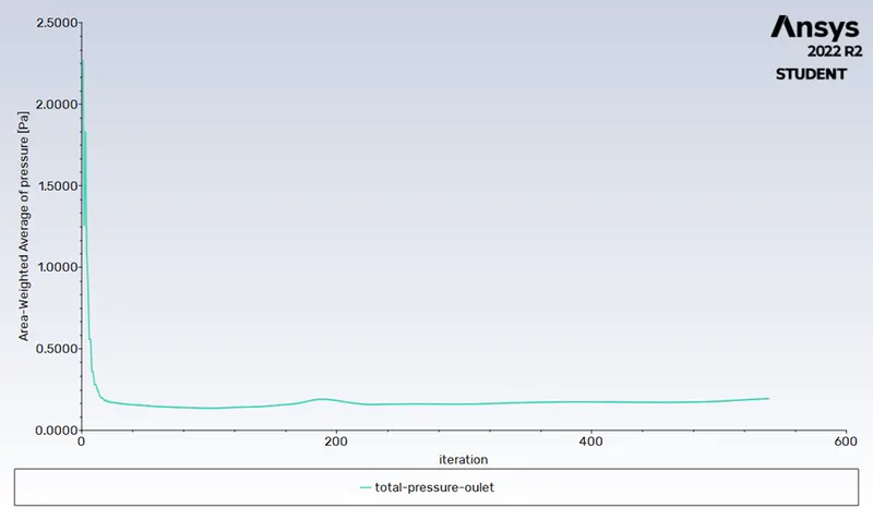
Pressure drop = Total pressure – Outlet pressure
Here we consider total pressure as inlet pressure and outlet pressure as top outlet pressure
We get Pressure drop = 1.9558 – 0.2170 = 1.7388 Pa
Separation efficiency = No. of Particle trapped/No. of Particle tracked
Then we got the efficiency as separation eff. = 269/288
Separation efficiency at 1m/s = 93.4%
Then export the particle data to post-process/result section to simulate and find out the flow of particle in cyclone separator and to simulate the problem with animation.
Post-process:
Import the particle data and enable the tracked particle move from cyclone separator, observe the particle exit at outlet (bottom) and outlet (top). Create the animation which provides the video of movement of particles in cyclone separator.
Anthracite particle floe in cyclone separator w.r.t time
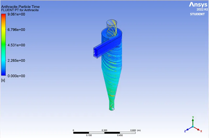
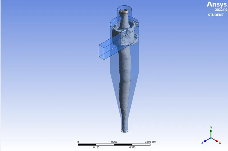
https://drive.google.com/file/d/1E112TuO34ersgDNDNxjWyjnSIDRmHsQQ/view?usp=share_link
Performing the simulation with particle diameter as 5micro meter at velocity of 2m/s:
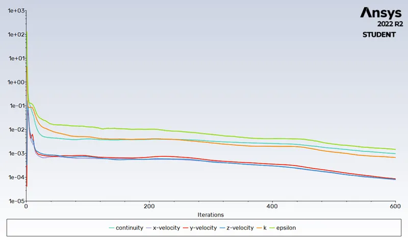
Residual plot:
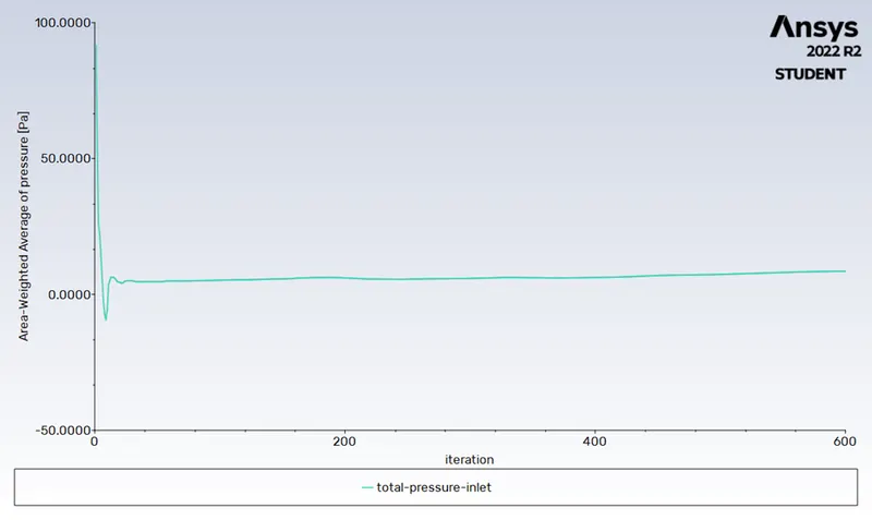
Pressure inlet:
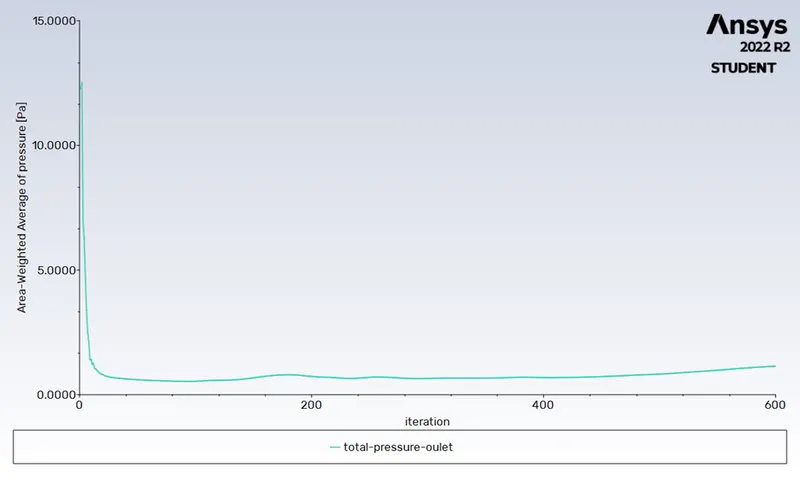
Pressure outlet:
Pressure drop = Total pressure – Outlet pressure
Here we consider total pressure as inlet pressure and outlet pressure as top outlet pressure
We get Pressure drop = 8.542 – 1.145 = 7.397 Pa
Separation efficiency = No. of Particle trapped/No. of Particle tracked
Then we got the efficiency as separation eff. = 282/288
Separation efficiency at 1m/s = 97.16%
Post-process:
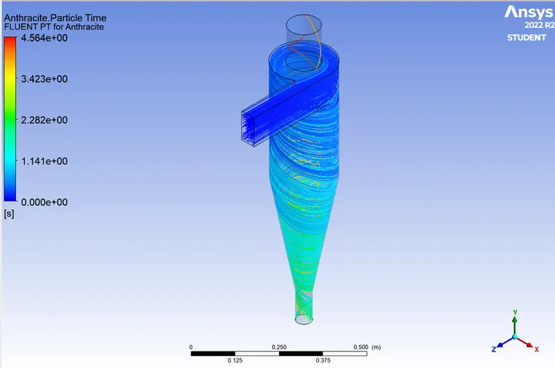
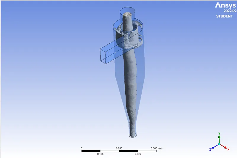
https://drive.google.com/file/d/153EFf6450WvJHt-wWAgw2WPDV2Zr5Pem/view?usp=share_link
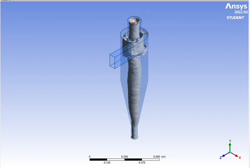
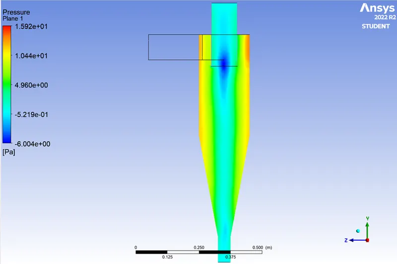
Performing the simulation with particle diameter as 5micro meter at velocity of 3m/s:
Residual plot:
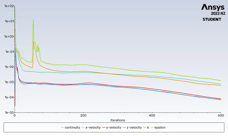
Pressure outlet:
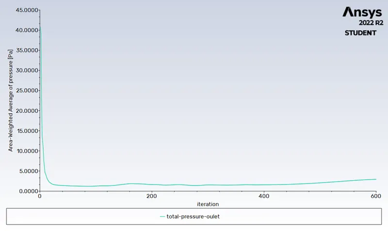
Pressure drop = Total pressure – Outlet pressure
Here we consider total pressure as inlet pressure and outlet pressure as top outlet pressure
We get Pressure drop = 20.183 – 2.947 = 17.236 Pa
Separation efficiency = No. of Particle trapped/No. of Particle tracked
Then we got the efficiency as separation eff. = 278/288
Separation efficiency at 1m/s = 96.52%
Post-process:
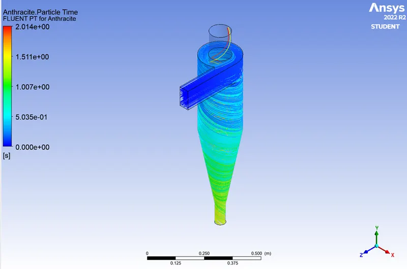
https://drive.google.com/file/d/1zJcAuKESFPL7_r1qy0M0hZTOr2dI8eDN/view?usp=share_link
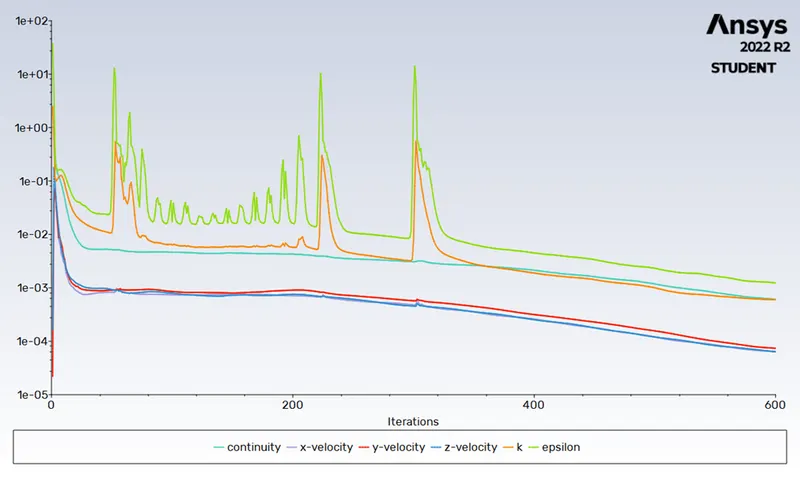
Performing the simulation with particle diameter as 5micro meter at velocity of 4m/s:
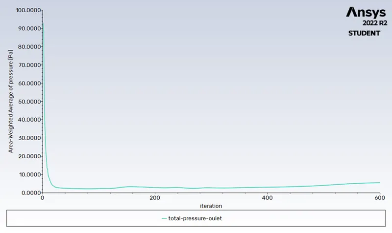
Residual plot:
Pressure inlet:
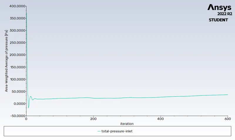
Pressure outlet:
Pressure drop = Total pressure – Outlet pressure
Here we consider total pressure as inlet pressure and outlet pressure as top outlet pressure
We get Pressure drop = 36.807 – 5.531 = 31.494 Pa
Separation efficiency = No. of Particle trapped/No. of Particle tracked
Then we got the efficiency as separation eff. = 274/288
Separation efficiency at 1m/s = 95.13%
Post-process:
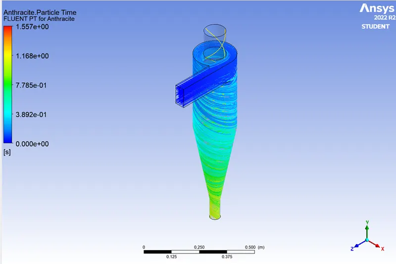
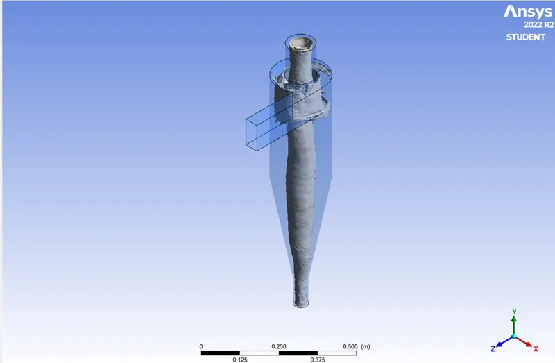
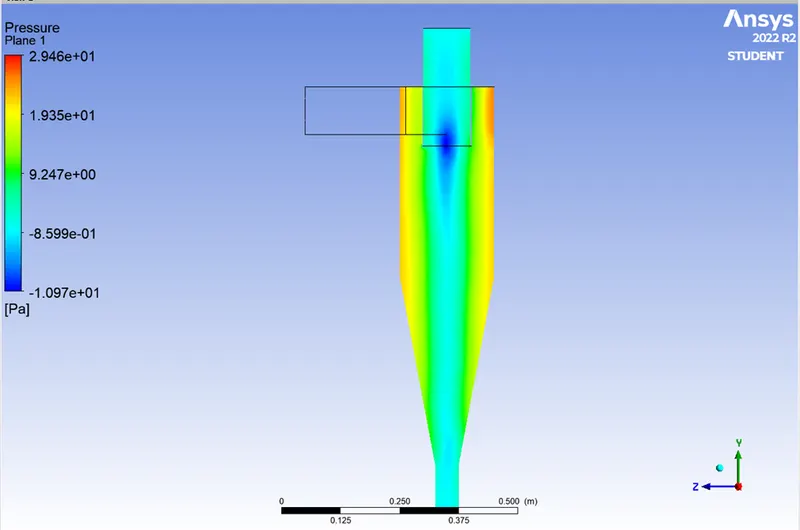
https://drive.google.com/file/d/1ChX6qJxNA_baWtAGpt6bzXuF67srR4bY/view?usp=share_link
Performing the simulation with particle diameter as 5micro meter at velocity of 5m/s:
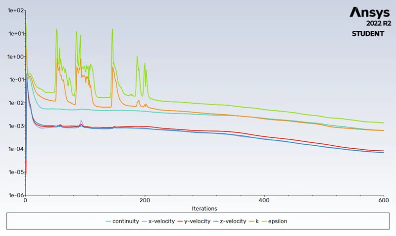
Residual plot:
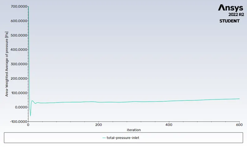
Pressure inlet:
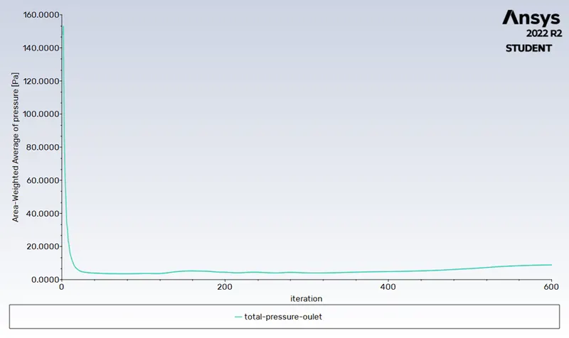
Pressure outlet:
Pressure drop = Total pressure – Outlet pressure
Here we consider total pressure as inlet pressure and outlet pressure as top outlet pressure
We get Pressure drop = 58.432 – 8.872 = 49.560 Pa
Separation efficiency = No. of Particle trapped/No. of Particle tracked
Then we got the efficiency as separation eff. = 253/288
Separation efficiency at 1m/s = 87.84%
Post-process:
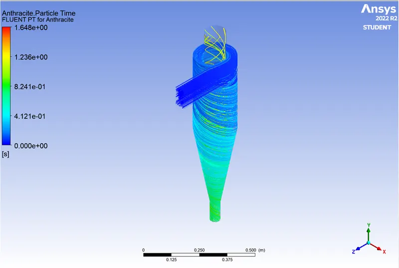
https://drive.google.com/file/d/1MhpFifKeLlqaiJCzQ5h4ibknPkyZhE1B/view?usp=share_link
Observations and Conclusion:
From case1 we say that as the diameter of particle increase the efficiency of separation also increases for cartesian mesh method and mesh size of 0.005m.
From case2 we seen that at constant particle diameter with variation of velocity the separation efficiency is increases till 3m/s velocity then after that 4&5 m/s of velocity the separation efficiency decreases coz the number of escape of particle is more as compare to first 3 velocity.
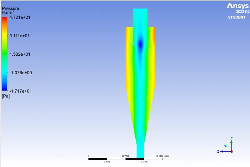
The Vortex Core Region results are similar for each test case. Therefore, it can be concluded that the particle diameter and velocity of injection do not play a role in the Vortex formed.
Increased velocity causes a higher pressure drop.