Week 8 - Simulating Cyclone separator with Discrete Phase Modelling
Aim: To perform analysis on the cyclone separator and calculate the separation efficiency and pressure drop.
Objective:
- Write a few words about any four empirical models used to calculate the cyclone separator efficiency.
- To perform an analysis on a given cyclone separator model by varying the particle diameter from 1 μm to 5 μm & calculate the separation efficiency in each case. Discuss the results. [Use both the velocity's as 3 m/sec.]
- To perform an analysis on a given cyclone separator model by varying the particle velocity from 1 m/sec to 5 m/sec and calculate the separation efficiency and pressure drop in each case. Discuss the results. [Use particle diameter size as 5 μm for all cases & keep flow velocity same as particle velocity]
Theory:
Cyclone separator
The Cyclone separator is a device used to remove particulate matter from air, gas, or water stream without the use of filters through vortex generation. The gravitational and centrifugal are the main forces responsible for the separation of particulate matter from fluid streams.
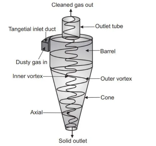
Cyclones are basically centrifugal separators. They simply transform the inertia force of the gas particle to a centrifugal force by means of a vortex generated in the cyclone body. The gas with particles enters tangentially at the upper part and passes through the body describing the vortex. Particles are driven to the wall by centrifugal forces, lose momentum and fall into the cyclone leg. In the lower section, the gas begins to flow radially inwards to the axis and spins upwards to the gas outlet duct.
The particles in the system experience changes in their momentum due to interaction with the separator geometry as well as exchange momentum, energy, and mass with the gas. The interaction with the gas phase might be in terms of buoyancy, drag, or viscous forces. To model this effectively, the Discrete Phase Modelling in Ansys Fluent is chosen.
Collection efficiency
The collection or separation efficiency is most properly defined for a given particle size. As mentioned, fractional efficiency is defined as the fraction of particles of a given size collected in the cyclone, compared to those of that size going into the cyclone. Basically, it is the ratio of particles trapped to the particles tracked.
Several equations have been developed to predict the collection efficiency in cyclones through correlation equations.
Empirical models:
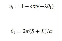
Iozia and Leith model - This model was developed based on force balance. In this model, since the particle undergoes vortex flow, two main forces are considered - i.e, centrifugal force and flow resistance.
The collection efficiency (ηi) of particle diameter (dpi) is given as-
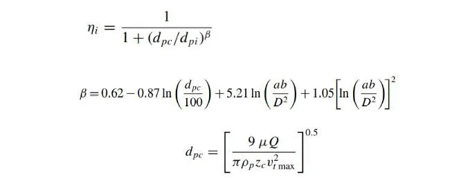
The model assumes that a particle carried by the vortex endures the influence of two forces: a centrifugal force (Z) and flow resistance (W), Core length (zc), and core diameter (dc).
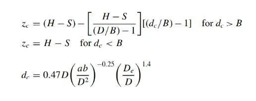
β is an expression for slope parameters derived based on the statistical analysis of experimental data of a cyclone with D = 170 and dpc is the 50% cut size given by Barth. where core length (zc) and core diameter (dc) are given as
Li and Wang model - This model includes particle bounce or re-entrainment and turbulent diffusion at the cyclone wall. In this model, a 2D analytical expression of particle distribution in the cyclone is given as-
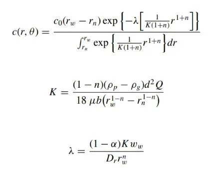
The resultant expression of the collection efficiency for particles of any size is given as-
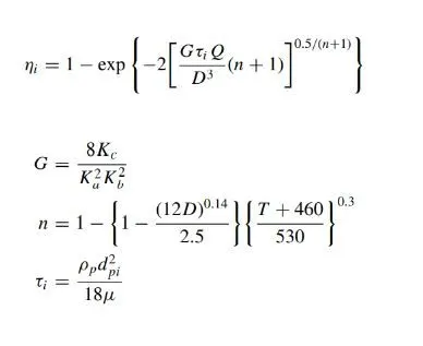
Koch and Licht model - This model includes the inherently turbulent nature of cyclones and the distribution of gas residence times within the cyclone.
A force balance and an equation on the particles collection yield the grade efficiency (ηi) as-
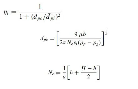
Lapple model - This model was developed based on force balance without considering the flow resistance. Lapple assumed that a particle entering the cyclone is evenly distributed across the inlet opening.
The efficiency of collection of any size of the particle is given by-
Procedure:
In this report, an analysis of the cyclone separator is performed in two different parts.
In part 1, the cyclone separator efficiency is computed for an inlet velocity of 3m/s with different particle diameter sizes.
In part 2, the cyclone separator efficiency is computed for a particle size of 5 micrometers with different inlet velocities.
In order to perform discrete phase modeling simulation, certain steps have to be followed.
Geometry
Choose the Fluid flow (fluent) module and start with editing geometry.
First import the cyclone separator cad model in space claim.
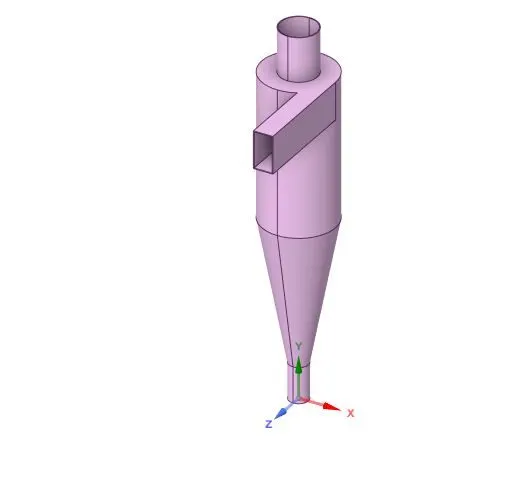
Next, extract the fluid volume inside the cyclone separator by Prepare -> Volume extract as shown in the fig and suppress the solid geometry.
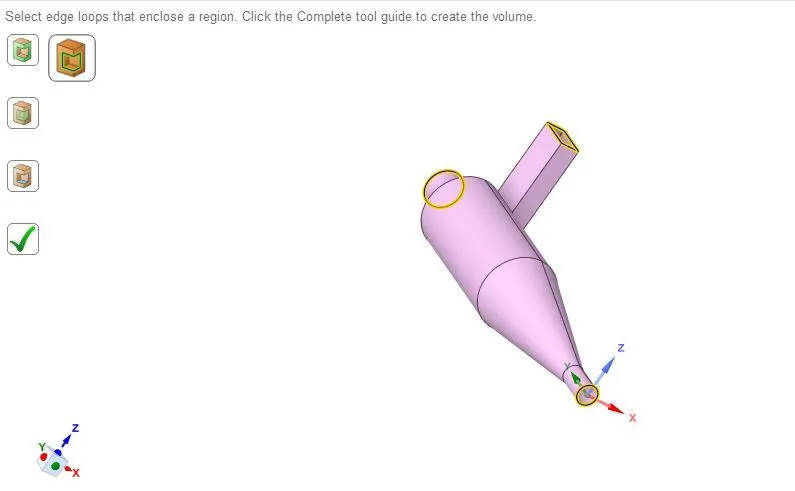
Figure: Pink geometry is the solid region (left) and the grey geometries are fluid regions prepared by using the volume extract tool in Ansys SpaceClaim.
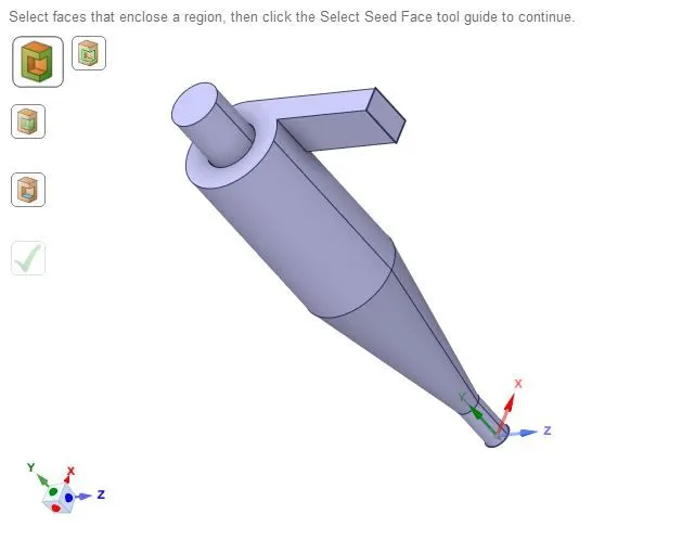
Fluid volume is extracted from the geometry by using the prepare option. so that we can analyze the fluid flow of the cyclone separator. Hide the previous geometry and suppress physics since we are only interested in the fluid flow and not the external surface.
Mesh
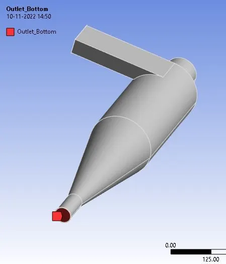
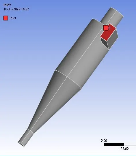
First, before generating the mesh, assign names to the parts and boundaries in the named selection as shown in the figure.
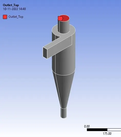
Named Selections
The face-selecting tool is selected. The inlets, outlet (top), and outlet (bottom) are named. The inlet is through which the particles enter the lighter impurities escape through the top, and the heavier impurities are trapped in the bottom.
Mesh stats:
1. Main element size = 10 mm
2. Method = Cartesian method
3. Cartesian element size = 10 mm
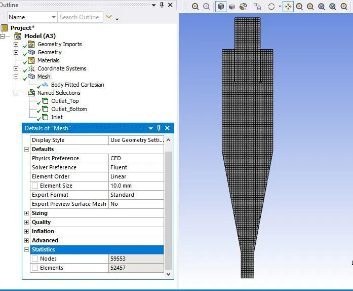
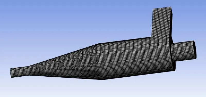
A body-fitted Cartesian mesh method is used to create the mesh. This method creates mesh with hexahedral elements. The hexahedral elements have the highest quality among all element types & give the most accuracy of solutions. The Cartesian mesh is generated using the coordinates of the Centroid of the model.
No of Nodes: 59553
No of Elements: 52457
Solution Approach & Solver Requirement
General conditions
This analysis involves the orientation of the cyclone separator. As it is in the x-y plane, the acceleration due to gravity needs to be turned on. As acceleration due to gravity acts upwards, the g value is assigned as -9.81 on the positive y-axis. Pressure based solver is used. The steady-state analysis is done and the velocity formulation is normal to the boundary and absolute.
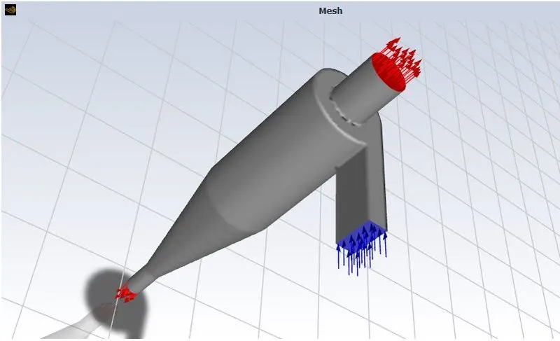
Solver type - Pressure based,
Velocity formulation - Absolute,
Time - Steady.
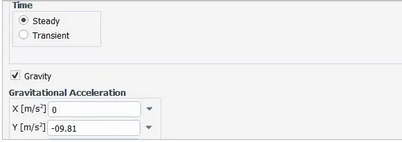
Physics setup: model
Turbulence modeling: The K-epsilon(2 equation) model with RNG and swirl-dominated flow is selected. The wall modeling functions are standard wall functions.
Since, in cyclone separators, turbulence dissipation effects play an important role, RNG K - epsilon turbulence model is used. RNG is a slight modification to standard K - epsilon, which increases the accuracy of swirling flows.
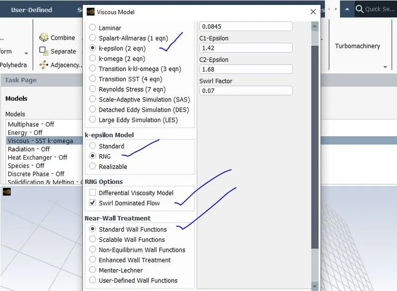
RNG k-epsilon is used in the viscous model.
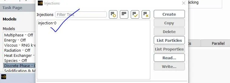
The discrete particles are introduced using the discrete phase model. Discrete phase modeling is used to track the flow of the particles.
The DPM iteration interval is the frequency with which the particles are tracked and the sources are updated.
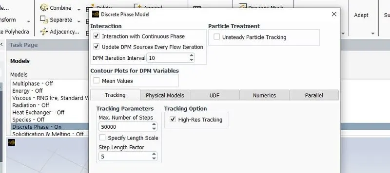
The model is enabled for interaction with the continuous phase. The DPM interval level is 10. For injection, the particle type is inert. From the fluent database, anthracite is selected. It is released from the inlet, with velocity in the x-direction being 3 m/s. This velocity may be manipulated further. The particle diameter chosen for the first analysis is one micrometer. The particle diameter is varied from 1 micrometer to 5 micrometers to calculate the separation efficiencies.
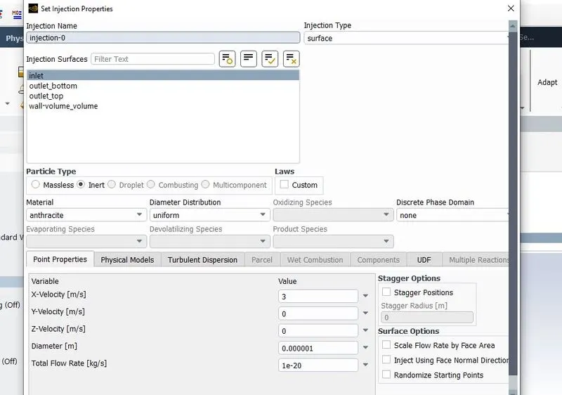
As discussed earlier, the Discrete Phase Modelling approach is used to simulate flow in the cyclone separator. This model follows the Euler-Lagrange approach. The fluid phase is treated as a continuum by solving the Navier-Stokes equations, while the discrete phase is solved by tracking a large number of particles.
It is assumed that the dispersed second phase occupies a low volume fraction. The particle trajectories are computed at specified intervals. Fluent predicts the particle trajectory by integrating the force balance on the particle, which is written in the Lagrangian frame.
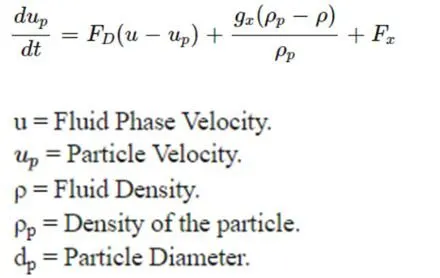
The coupling between the continuous and the discrete phase is done using two-way coupling. The continuous phase influences the discrete phase via drag and turbulence. The discrete phase via source terms of mass, momentum, and energy.
The tracking parameters used to control the time integration of the particle trajectory equation are;
Maximum number of steps: - Imposes a limit on the number of time steps to avoid the possibility of a particle being trapped in a recirculating region of the continuous phase. If the particle never exits the flow, it is reported as ‘incomplete’.
Length scale & Step length factor: - The integration time step is computed based on a specified length scale & the velocity of the particle & continuous phase. It is equivalent to the distance that the particle will travel before its motion equations are solved again & its trajectory is updated.
The step length factor allows Fluent to compute the time step in terms of the number of time steps required for a particle to traverse a computational cell. One thumb rule to follow is if a particle is to advance through N mesh cells in the main flow direction, the step length factor times N should be approx equal to the max number of steps.
Boundary Conditions
The boundary conditions are provided to three named selections:
Inlet and wall - Reflect
Outlet(Top) - Escape
Outlet(Bottom/dustbin) - Trap
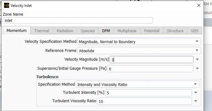
For the inlet, the momentum conditions are velocity is 3m/s in the x-direction, being absolute and normal to the boundary. The DPM condition is set to reflect. This signifies that the particles are not allowed to escape or get trapped in the inlet.
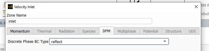
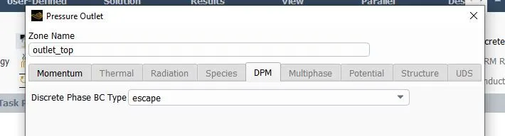
For the top outlet, the Momentum condition is the pressure condition, The DPM condition is set to escape. Particles can escape from this Boundary.
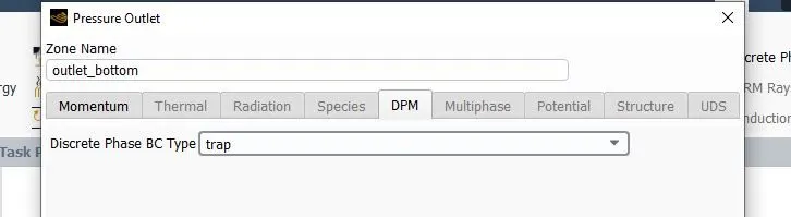
The bottom outlet is also a pressure outlet, with the DPM condition being trapped.
Wall type - no slip conditions, magnitude = zero gauge, and reflect type
Here above all boundary conditions, we have given different DPM conditions like Reflect, Escape, and Trap.
Reflect: It is the Particle Rebound off the boundary in question with a change in its momentum as defined by the coefficient of restitution.
Escape: The particle is reported as having “escaped” when it encounters the boundary in question. Trajectories calculated are terminated.
Trap: The Trajectory calculated is terminated and the fate of the particle is recorded as “trapped”. In the case of evaporating droplets, their entire mass instantaneously passes into the vapor phase and enters the Cell adjacent to the boundary. In the case of combusting particles, the remaining volatile mass is passed into the vapor phase.
Solution methods
The pressure velocity coupling is chosen as COUPLED scheme. The gradient is least-square cells based. Pressure, Momentum, Turbulent kinetic energy, and turbulent dissipation rate are second-order upwind.

Initialization
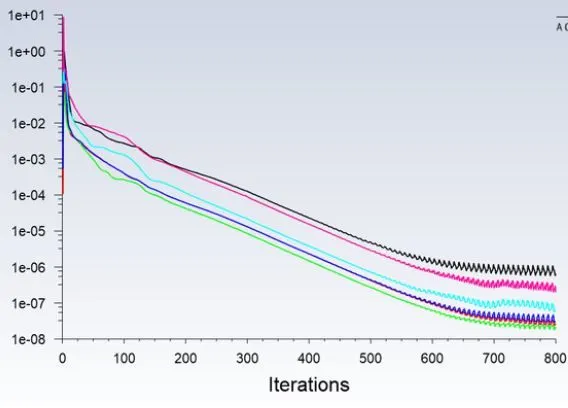
Standard initialization is done with flow from inlets for 800 iterations
In this part, we are making the velocity constant and we are visualizing the difference in results for different particle sizes.
Results:
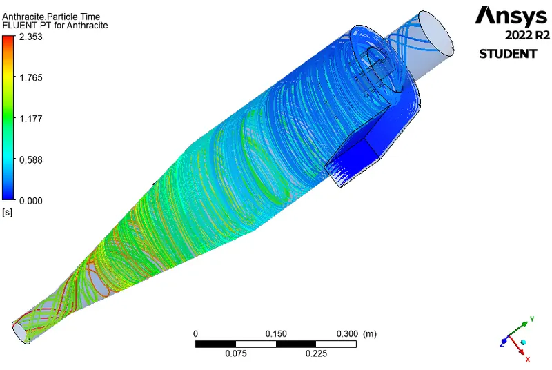
In CFD POST, in order to visualize the particle tracking data, import the file by File -> Import -> Import fluent particle track file.
Results for the particle size of 1 micrometer with a velocity of 3 m/s
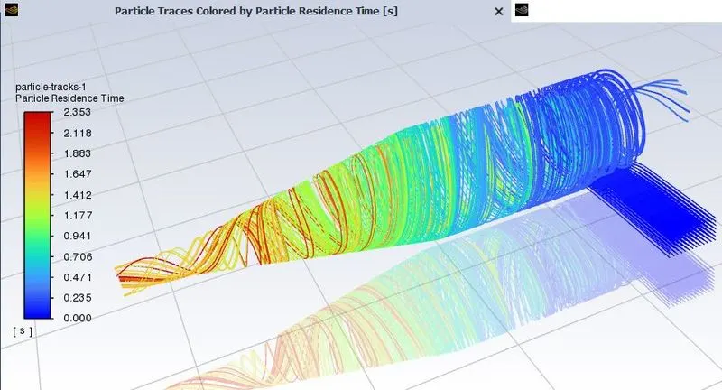
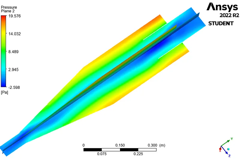
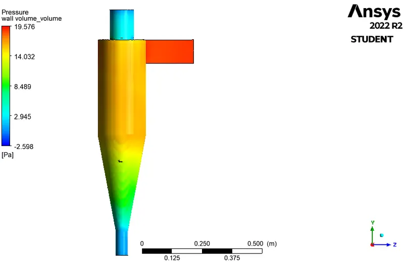
The following fig shows the particle time and particle pressure contours. A total of 98 particles are tracked.

Post-Processing:
Pressure plane
Results for the particle size of 3 micrometers with a velocity of 3 m/s
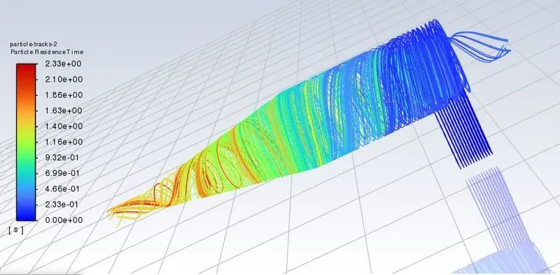
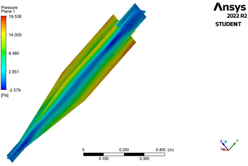
The following fig shows the particle time and particle pressure contours. A total of 91 particles are tracked.

Post-Processing:
Pressure plane
Results for the particle size of 5 micrometers with a velocity of 3 m/s
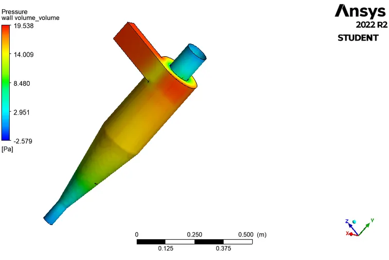
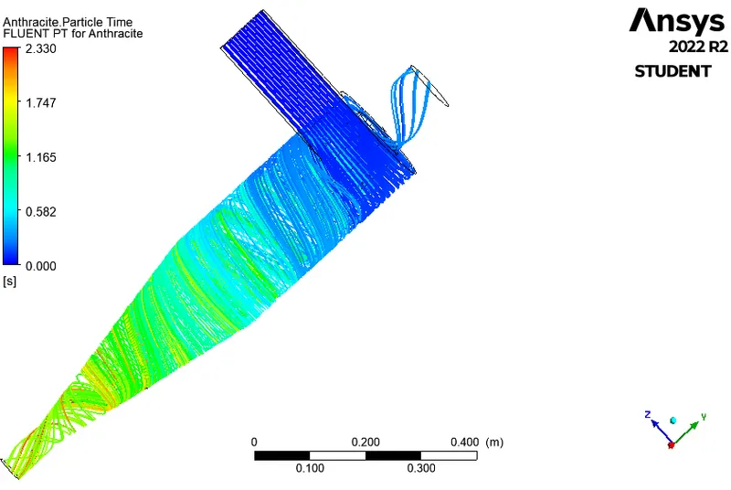
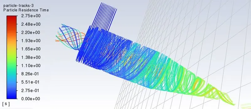
The following fig shows the particle time and particle pressure contours. A total of 98 particles are tracked.
Post-Processing:
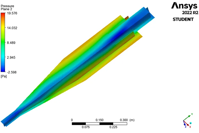
Pressure plane
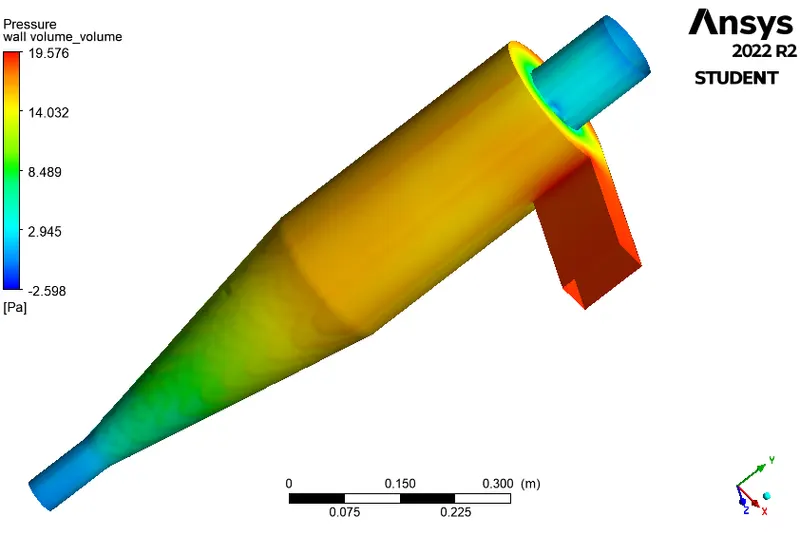
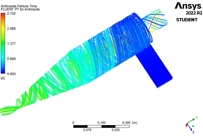
From the obtained results Separation efficiency and pressure drop are studied.
Separation efficiency: It is defined as the fraction of particles of a given size collected in the cyclone, compared to those of that size going into the cyclone. Experience shows that the separation efficiency of the cyclone separator increases with increasing particle mean diameter and density; increasing gas tangential velocity; decreasing cyclone diameter; increasing cyclone length; extraction of gas along with solids through the cyclone legs. In this case, depending on the particle history data - Separation Efficiency is defined as the ratio of concentration that has been removed from the feed stream to the initial concentration in the feed stream. For this case ratio of the number of trapped particles to the total number of particles tracked.
Cyclone separator efficiency = no.of particles trapped / no.of particles tracked
Pressure Drop: Pressure drop across the cyclone is of much importance in a cyclone separator. The pressure drop significantly affects the performance parameters of a cyclone. The total pressure drop in a cyclone will be due to the entry and exit losses, and friction and kinetic energy losses in the cyclone. Normally the most significant pressure drop occurs in the body due to swirl and energy dissipation. Pressure drop is defined as the difference in total pressure between two points of a fluid-carrying network.
Pressure drop = Total inlet pressure - Total Outlet Pressure
As the “escape” DPM condition is given to the outlet-top in this case, so outlet-top is considered in the pressure drop calculation.
Pressure drop occurs because of the following components:
Loss due to the expansion of gas in the cyclone chamber.
Loss due to rotational kinetic energy.
Loss due to wall frictional forces
Table:
| Element size (micrometer) | Number of tracing elements | Number of trapped elements | Number of escaped elements | Cyclone separator efficiency (%) |
| 1 | 98 | 52 | 38 | 53.06 |
| 3 | 98 | 75 | 23 | 76.53 |
| 5 | 98 | 94 | 04 | 95.91 |
Results:
The fluid velocity & particle velocity are 3 m/sec for all particle sizes remaining the same in Part1. Therefore the pressure drop remains constant for all analyses of Part1.
The collection efficiency of the cyclone separator is related to the pressure drop across the cyclone. Here pressure drop is the indirect measure of the energy required for the gas to move the particles. Pressure drop is related to the inlet velocity of air and particle size.
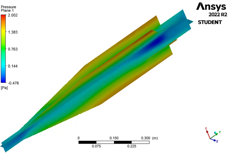
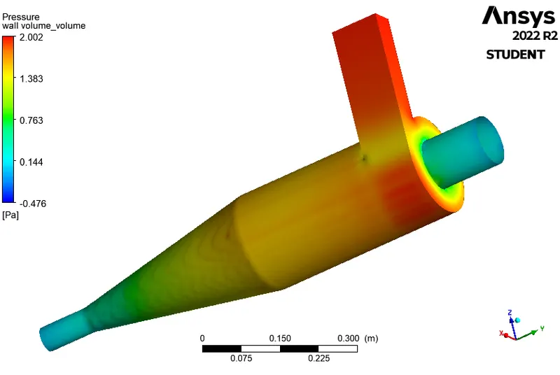
From the above pressure velocity plots, we can infer that the pressure is higher near the wall region which forms the outer vortex.
Due to higher pressure near the wall low-pressure region is created at the center of the cyclone separator because of which the lighter particles escape from the top outlet and heavier particles are collected at the bottom outlet.
Part 2
Particle diameter size = 5 microns and varying inlet velocity = 1 m/s, 3 m/s, & 5 m/s.
Results for the particle size of 5 micrometers with a velocity of 1 m/s
Residual plot:
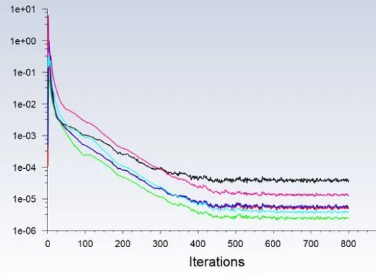
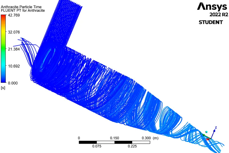
The following fig shows the particle time and particle pressure contours. A total of 98 particles are tracked.

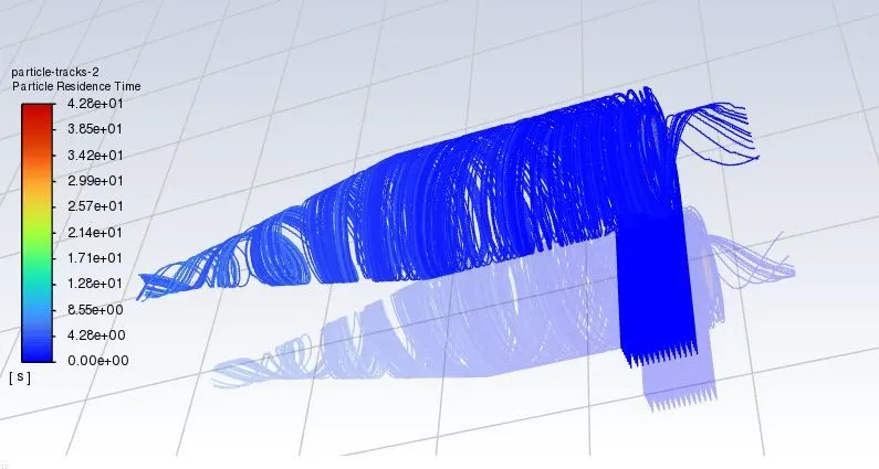
Post-Processing:
Pressure plane
Results for the particle size of 5 micrometers with a velocity of 3 m/s
Residual plot:
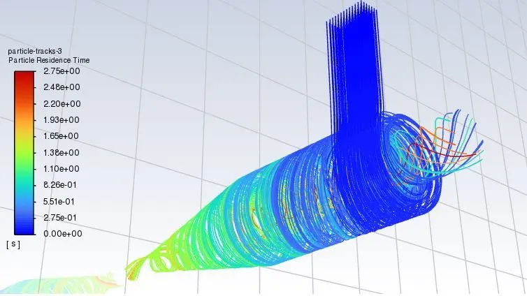
The following fig shows the particle time and particle pressure contours. A total of 98 particles are tracked.

Post-Processing:
Pressure plane
Results for the particle size of 5 micrometers with a velocity of 5 m/s
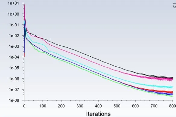
Residual plot:
The following fig shows the particle time and particle pressure contours. A total of 98 particles are tracked.
Post-Processing:
Pressure plane
Table:
| Inlet velocity (m/s) | Number of tracing elements | Number of trapped elements | Number of escaped elements | Cyclone efficiency (%) |
| 1 | 98 | 7 | 24 | 7.14 |
| 3 | 98 | 89 | 9 | 90.81 |
| 5 | 98 | 96 | 02 | 97.95 |
Results:
As the inlet velocity increases, the total pressure drop in the cyclone separator increases. So, it can be estimated that the energy losses increase with the increase in the inlet velocity.
For 1 m/s particle velocity, the vortex formed has lesser strength as compared to 3 m/s particle velocity. In fact, as the particles reach the cone, some drop straight down into the outlet bottom without following a curved trajectory.
The pressure contour shows a uniform distribution in the barrel & cone section whereas a negative pressure zone at the outlet top for 1 m/s particle velocity. This pressure gradient drives the particles toward the top at the outlet bottom.
Conclusion:
From the table, it can be observed that as the velocity increases the cyclone efficiency increases, and the particle diameter size is increased. The pressure drop inside the cyclone separator increases when the inlet velocity is increased and the particle size doesn't affect the pressure drop inside the cyclone separator.
It can be observed from the contours that as the velocity increases the radial pressure drop increases. Thus more the pressure drop, more is the cyclone efficiency.
From the results, it is observed that heavier particle is trapped at the bottom outlet and lighter particles are escaped at the outlet top. But we can also see that lighter particles also get trapped at the bottom outlet because of interaction between lighter and heavier particles and there is an exchange of inertial forces between them as a result there is a transfer of Kinetic energy from heavier particles to the lighter particle, as a result, we can observe a certain number of heavier particles escapes through the top outlet.
The collection efficiency of cyclones varies as a function of particle size, density, & cyclone design. Cyclone efficiency will generally increase with the increase in particle size, density, inlet duct velocity, cyclone body length, number of gas revolutions in the cyclone, the ratio of cyclone body diameter to gas exit diameter, inlet dust loading, smoothness of the cyclone inner wall.
The efficiency of the cyclone will decrease with an increase in the parameters such as gas viscosity, cyclone body diameter, gas exit diameter, gas inlet duct area, gas density, and leakage of air into the dust outlet. With the increase in inlet velocity or particle size the efficiency increases.
Research Papers: