Week 8 - Simulating Cyclone separator with Discrete Phase Modelling

SIMULATION OF CYCLONE SEPARATOR EFFICIENCY AND PRESSURE DROP CALCULATION

Introduction:

The main aim of this study is to calculate the emphasis of temperature, operating pressure and inlet velocity on the separator efficiency of a cyclone separator. Typically cyclone separators are used in cement industries to filter the embedded solid particles from a gas phase. CFD analysis is the tool used to predict the efficiency and operation capacity parameters of a particular geometry cyclone separator. The study is also used to predict the maximum diameter of the particles the cyclone is able to separate with the same efficiency.

Discrete Phase Modelling:

The discrete phase modelling is a sub section of Muliphase flows. A DPM is used when the aim is to investigate the behaviour of the particles from a Lagrangian view and a discrete perspective. The difference between the Lagrangian and Eulerian view is that fluid behaviour in the Lagragian view is examined based in particle tracking of a particulate flow, whereas fluid behaviour is considered in the Eulerian view based on the assumption of a finite volume element in the fluid flow path.

In DPM, the continuous phase is solved using Navier-Stokes equations. At the same time, the discrete phase is simulated by tracking a large number of particles, bubbles or droplets passing through the calculated continuous flow field. It should be noted that the discrete phase can exchange momentum, mass and energy with the continuous phase. This method can be made much simpler by ignoring the interaction of particles with each other. Of course, this can happed when the discrete phase, even with a large mass, has a much smaller volume (less than 10%) than the continuous phase calculations, the particle paths are calculated and determined separately.

The RNG K-Epsilon model is a convenient model for simulating jet impingement, swirling flows, secondary flows and separation flows. yet the isotropic eddy viscosity assumption holds a disadvantage at times.

Cyclone separator:

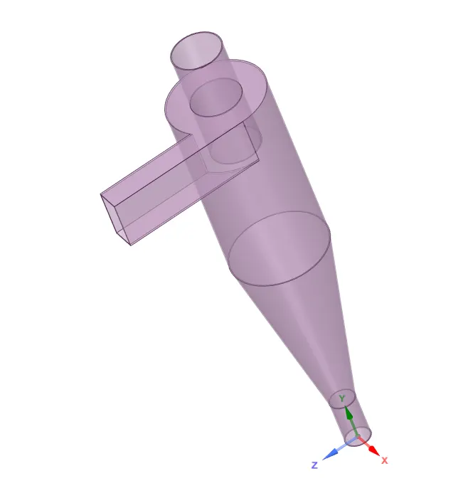
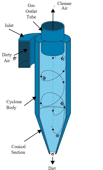
A cyclone separator is an economical device for removing particulate solids from a fluid system. The induced centrifugal force is tangentially imparted on the wall of the cyclone cylinder. This force with the density difference between the fluid and solid increases the relative settling velocity. It is also called as water scrubber or bag-house filter system, and related to an electrostatic precipitator. The dry cyclone can remove up to 100 micron size particles. Dust gets loaded in the flue gas. Usage of a water scrubber after the cyclone effectively removes all the dust particles. In commercial applications, both Electrostatic precipitator and bag-house filter systems are used. Adjusting the migration velocity and specific collection area increases the efficiency.

The efficiency of a cyclone separator:

The efficiency of the cyclone separator depends on the particle property which needs to be separated. Particles with diameter 5micrometers can be separated with an efficiency percentage of more than 95%. More the deviation with the particle size, more difference with the efficiency is observed. Flue gases with suspended particles is seen with the most efficient separation by the cyclone. Material property such as sticky or cohesiveness also has some influence on the efficiency. Here Anthracite particles are used as it is the most convenient particle to be used to study the working of the cyclone.

For a CFD simulation, the efficiency of separation can be calculated by the formula;

`eta=`Number of particles trapped/Number of particles tracked.

Empirical models used for cyclone separator efficiency calculation:

Lozia and Leith model:

It is a modified version od Barth 1956 model which is developed based on force balance. The model assumes that a particle carried by vortex endures the influence of two forces - a centrifugal force Z and a flow resistance W, Core length zl and core diameter d, which is given by

`zl = (H-S) -[(H-S)/((D/B)-1)] [(d/B_-1)]` for d>B

zl = (H-S) for d<B

`d=0.47 ((ab)/D^2)^(-0.25) (d/D)^1.4`

The addition made by lozia and leith on the original Barth 1956 model are the core length Zl and the shape parameter `beta`expression which is derived based on the statistical analysis of experimental data of cyclone with D=0.25m. The collection efficiency `eta`of particle diameter dp can be calculated from

`eta = (1/(1+(dpc)/(dp))^beta)`

where dpc is the 50% cut size given by Barth 1956 model, given by

`dpc=[(9muQ)/(pi P zlv^2 max) ]^0.5`

Li and Wang model:

The Li and Wand 1989 model includes particle bounce or re-entrainment and turbulent diffusion at the cyclone wall. A two-dimensional analytical expression of particle distribution in the cyclone is obtained. Li and Wang model was developed based on the assumptions that,

1.The radial particle velocity and the radial concentration profile are not constant, for uncollected particles within the cyclones.

2.Boundary conditions with the consideration of turbulent diffusion coefficient and particle bounce re-entrainment on the cyclone wall are:

C=Co, at `theta=0`

`D (del c)/(delr) = (1-alpha)wc,`at r=D/2

The tangential velocity is related to the radius of cyclone by

`uR^n = constant`

The concentration distribution in a cyclone is given as:

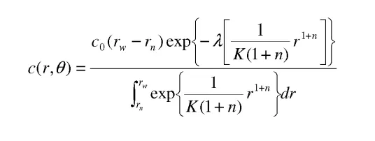
where `k=((1-n)(rhon-rhog)d^2Q)/(18mub(rw^(1-n) - rn^(1-n))`

and

`lamda = ((1-alpha)kw)/(D rw^n)`

The resultant expression of the collection efficiency for particle of my size is given as

`eta = 1-exp{-lamda theta}`

where `theta = (2pi (S+L))/alpha`

KOCH AND LICHT MODEL:

This theory recognized the inherently turbulent nature of cyclones and the distribution of gas residence times within the cyclone. Koch and Licht describe particle motion in the entry and collection regions with the additional assumptions like:

The tangential velocity of a particle ie equal to the tangential velocity of the gas flow. There is no slip in the tangential direction between the particle and the gas.

The tangential velocity is related to the radius of cyclone by:

`uR^n = constant`

A force balance and an equation on the particles collection yields the grade efficiency `eta`

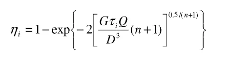
where `G=(8kc)/(ka^2. kb^2`

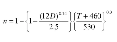
`taui=(rhop .dp^2)/(18mu)`

G is a factor related to the configuration of the cyclone, n is related to the vortex and `tau`is the relaxation term.

Lapple model:

This model is based on force balance without considering the flow resistance. Lapple assumed that a particle entering the cyclone is evenly distributed across the inlet opening. The particle that travels from inlet half width to the wall in the cyclone is collected with 50% efficiency. The semi elliptical relationship developed by Lapple to calculate a 50% cut diameter dp, is

`dp=[(9mub)/(2iNv(rhop-rhog))]^(1/2)`

where N is the number of revolutions.

`N=1/a[(h+(H-h)/2)]`

The efficiency of collection of any size particle is given by

`eta = 1/(1+((dp)/(di))^2`

Setup:

Step 1: Setting up geometry

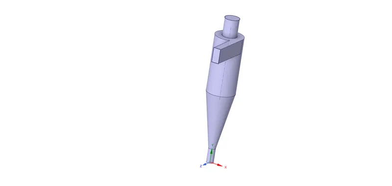
The cyclone separator geometry is imported in the SpaceClaim component.

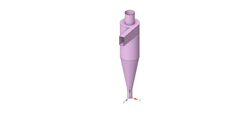
Using volume extract, select edges tool, fluid volume is extracted.

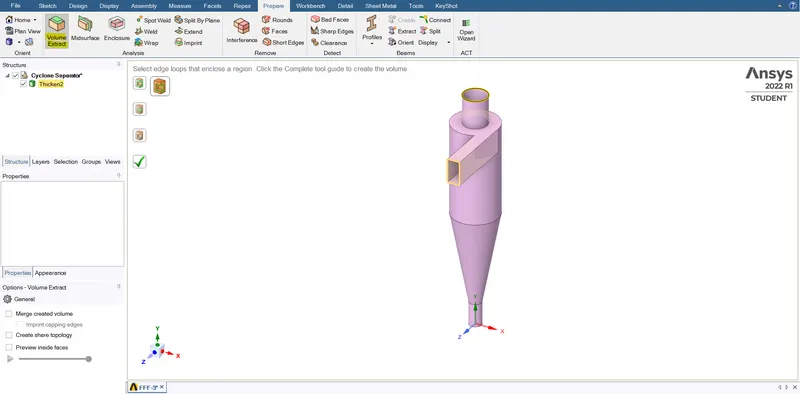
The extracted fluid volume is loaded and checked for interference and extra edges.

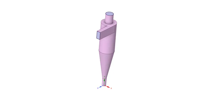
The volume other than fluid volume is suppressed for physics, and the remaining volume is transported to meshing.

Step 2: Meshing

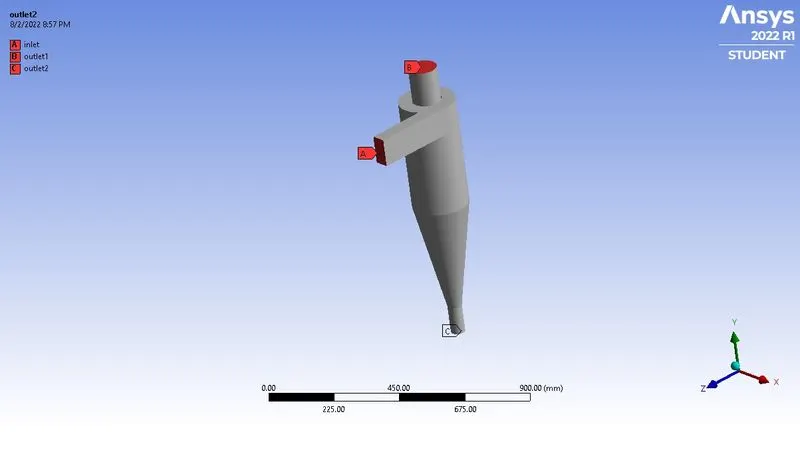
The fluid volume alone is selected for meshing. The inlet and the outlets are named in the volume.

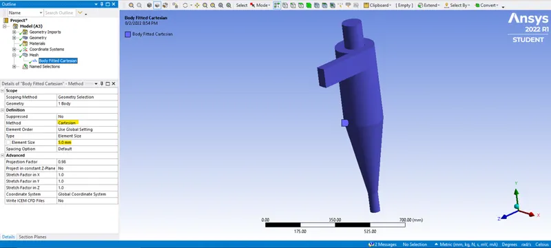
A cartesian mesh method is selected for the fluid volume.

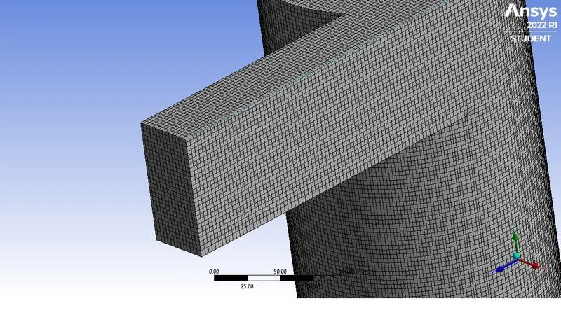
The inlets are checked for mesh quality

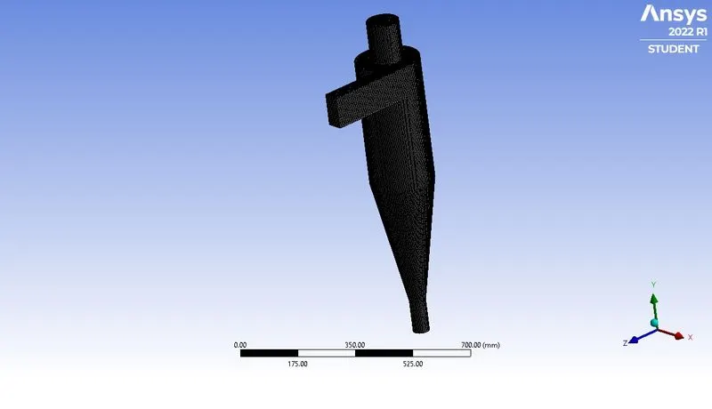
The total number of cells generated and interference is checked, as the meshing should be done only for the fluid volume by suppressing the solid volume interfaces.

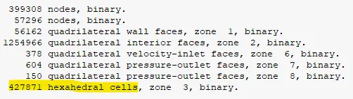
Step 3: Setting up the fluent environment

The basic solver setup and the model setup is done to startoff the fluent setup. The RNG K-Epsilon model is selected with swirl dominated flow solver.

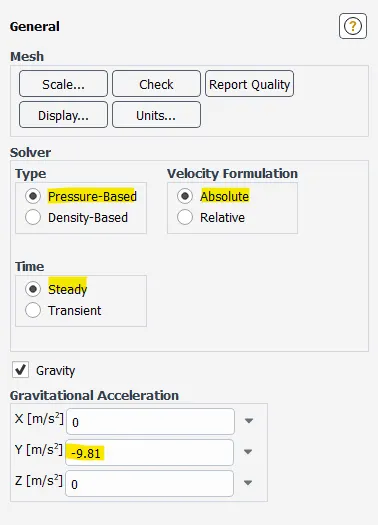
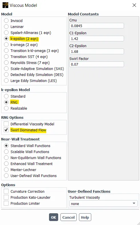
The Discrete Phase Model is set with injections from x-axis inlet, anthracite material, diameter and flow velocity is also set. The DPM iteration interval is set between 1 to 10.

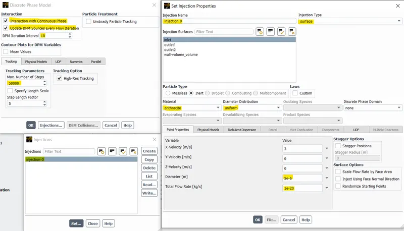
The Boundary conditions is set for 1 inlet and 2 outlets. The DPM conditions are also set for the inlets and outlets.

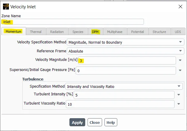
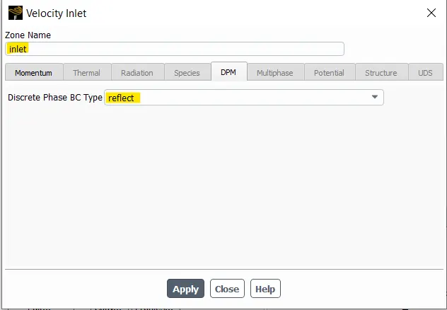
Boundary conditions:

Inlet: Reflect

Outlet 1: Escape

Outlet 2: Trap

Total flow rate: 1e-20 kg/s

Run Cases:

Part 1: In the first part of the simulation, the flow and inlet velocities are maintained the same at 3m/s, while the particle diameter is varied from 1`mum` to 5`mum`, to calculate the efficiency. The DPM iteration interval is set between 1 to 10 for different cases to reduce the incomplete particle levels.

Case 1.1	Case 1.2	Case 1.3	Case 1.4	Case 1.5
Flow velocity = 3m/s Inlet velocity = 3m/s Particle diameter = 1`mum`	Flow velocity = 3m/s Inlet velocity = 3m/s Particle diameter = 2`mum`	Flow velocity = 3m/s Inlet velocity = 3m/s Particle diameter = 3`mum`	Flow velocity = 3m/s Inlet velocity = 3m/s Particle diameter = 4`mum`	Flow velocity = 3m/s Inlet velocity = 3m/s Particle diameter = 5`mum`

Part 2: This time, the particle diameter is set constant at 5`mum` and the flow and inlet velocities are varied from 1m/s to 5m/s to calculate the efficiency. The DPM iteration interval is set between 1 to 10 for different cases to reduce the incomplete particle levels.

Case 2.1	Case 2.2	Case 2.3	Case 2.4	Case 2.5
Particle diameter = 5`mum` Flow velocity = 1m/s Inlet velocity = 1m/s	Particle diameter = 5`mum` Flow velocity = 2m/s Inlet velocity = 2m/s	Particle diameter = 5`mum` Flow velocity = 3m/s Inlet velocity = 3m/s	Particle diameter = 5`mum` Flow velocity = 4m/s Inlet velocity = 4m/s	Particle diameter = 5`mum` Flow velocity = 5m/s Inlet velocity = 5m/s

Results:

Residuals plot:

Case 1.1 (D=1`mum`)	Case 2.1 (Vi=Vf=1m/s)
Case 1.2 (D=2`mum`)	Case 2.2 (Vi=Vf=2m/s)
Case 1.3 (D=3`mum`)	Case 2.3 (Vi=Vf=3m/s)
Case 1.4 (D=4`mum`)	Case 2.4 (Vi=Vf=4m/s)
Case 1.5 (D=5`mum`)	Case 2.5 (Vi=Vf=5m/s)

Pressure contour:

Case 1.1 (D=1`mum`)	Case 2.1 (Vi=Vf=1m/s)
Case 1.2 (D=2`mum`)	Case 2.2 (Vi=Vf=2m/s)
Case 1.3 (D=3`mum`)	Case 2.3 (Vi=Vf=3m/s)
Case 1.4 (D=4`mum`)	Case 2.4 (Vi=Vf=4m/s)
Case 1.5 (D=5`mum`)	Case 2.5 (Vi=Vf=5m/s)

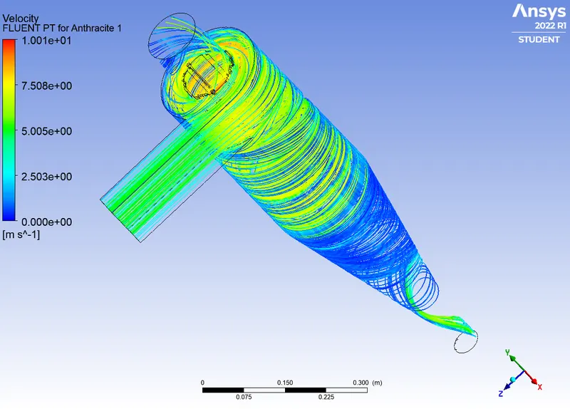
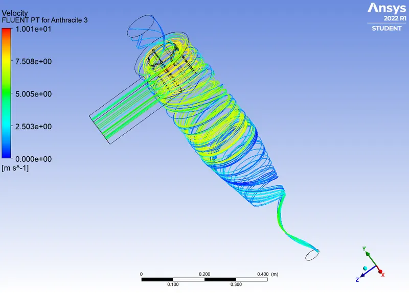
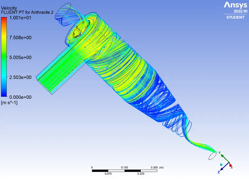
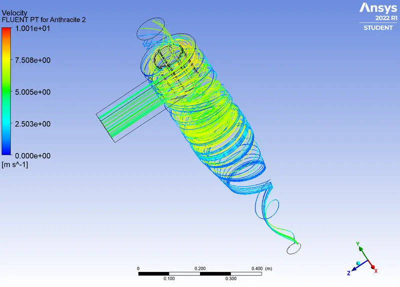
Velocity contour:

Case 1.1 (D=1`mum`)	Case 2.1 (Vi=Vf=1m/s)
Case 1.2 (D=2`mum`)	Case 2.2 (Vi=Vf=2m/s)
Case 1.3 (D=3`mum`)	Case 2.3 (Vi=Vf=3m/s)
Case 1.4 (D=4`mum`)	Case 2.4 (Vi=Vf=4m/s)
Case 1.5 (D=5`mum`)	Case 2.5 (Vi=Vf=5m/s)

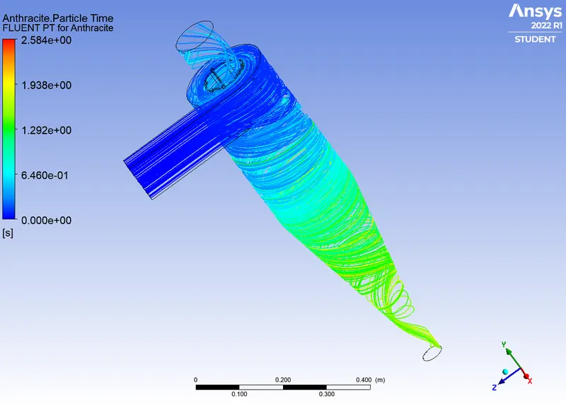
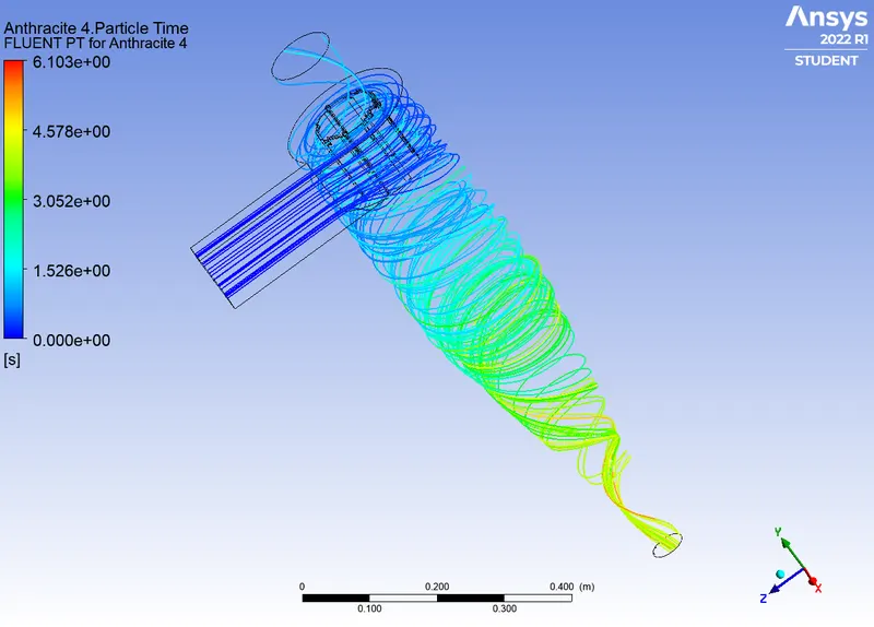
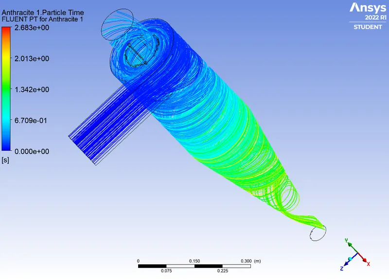
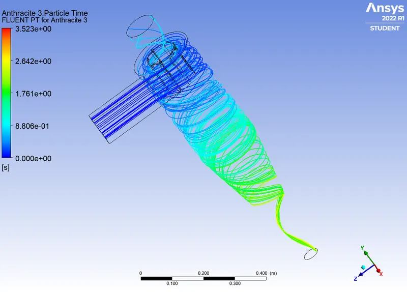
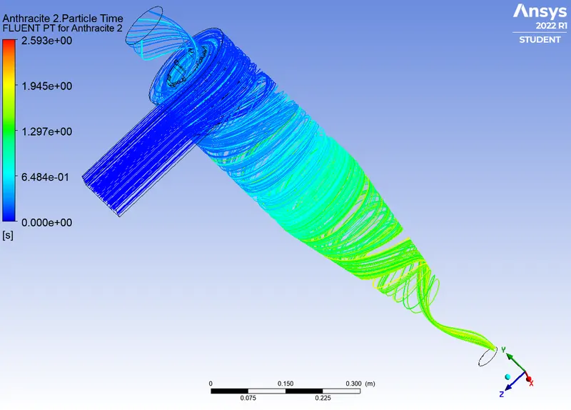
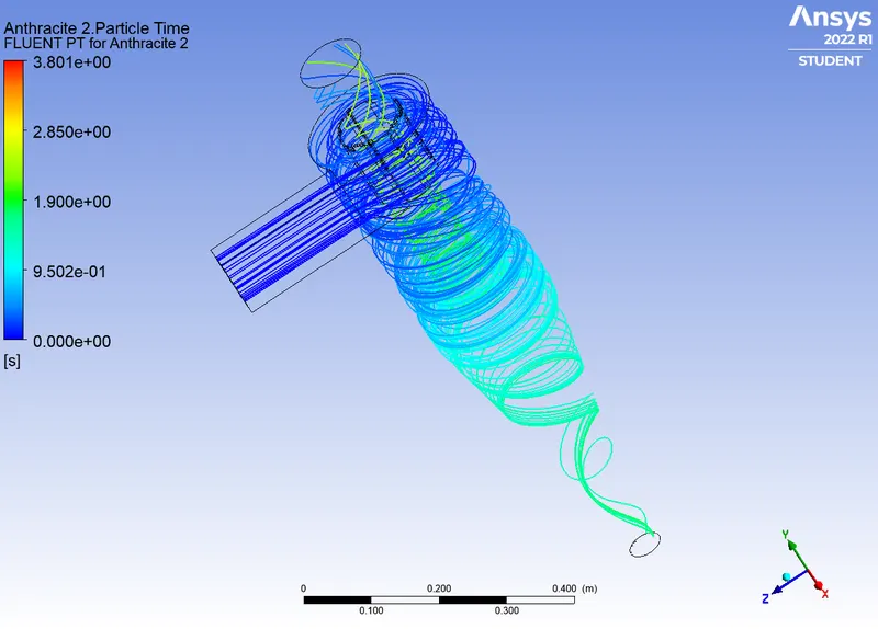
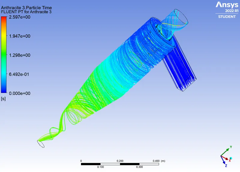
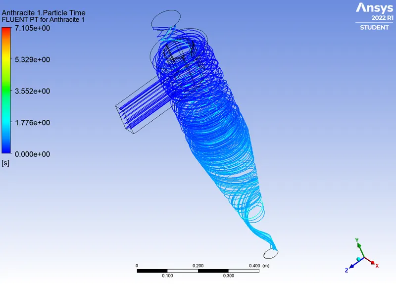
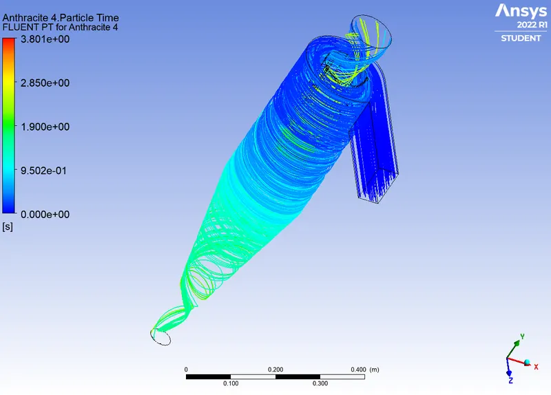
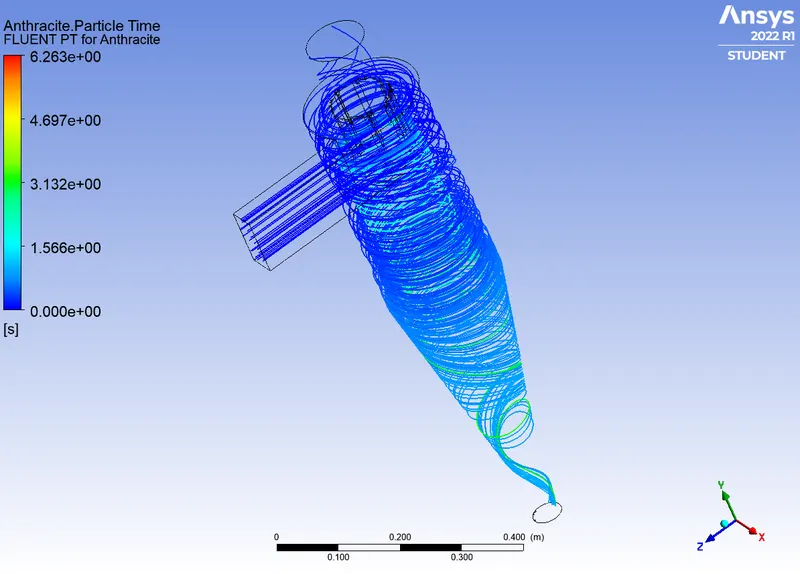
Particle time contour:

Case 1.1 (D=1`mum`)	Case 2.1 (Vi=Vf=1m/s)
Case 1.2 (D=2`mum`)	Case 2.2 (Vi=Vf=2m/s)
Case 1.3 (D=3`mum`)	Case 2.3 (Vi=Vf=3m/s)
Case 1.4 (D=4`mum`)	Case 2.4 (Vi=Vf=4m/s)
Case 1.5 (D=5`mum`)	Case 2.5 (Vi=Vf=5m/s)

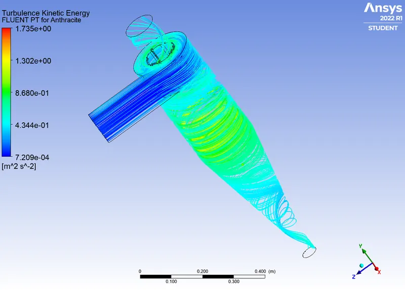
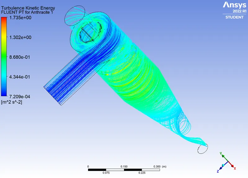
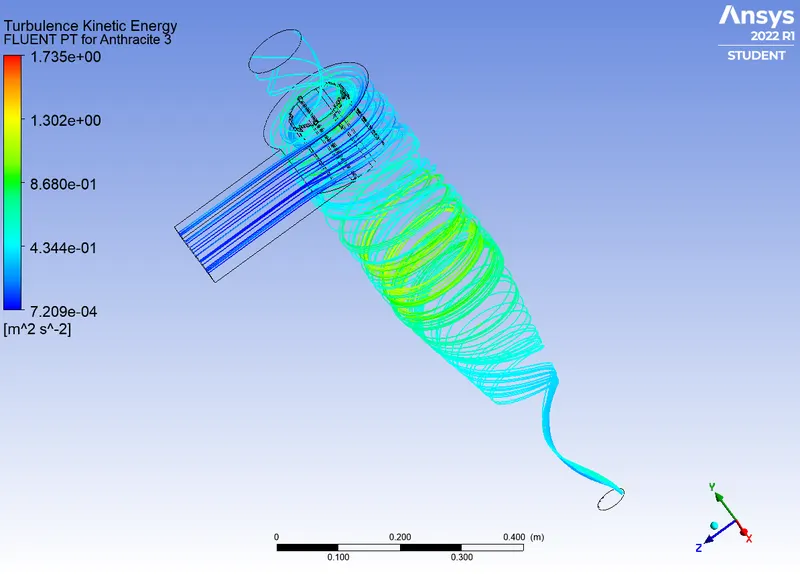
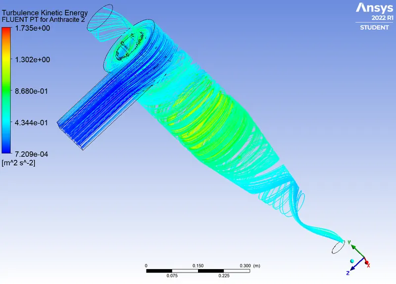
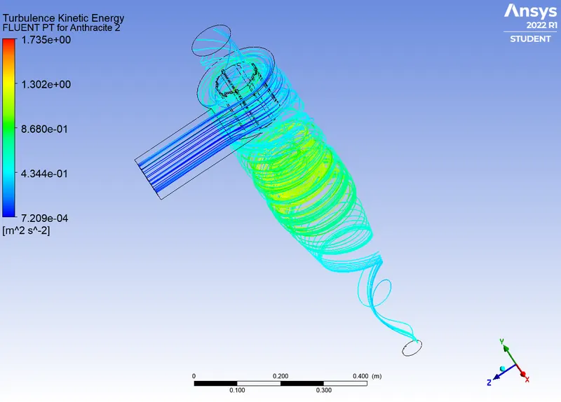
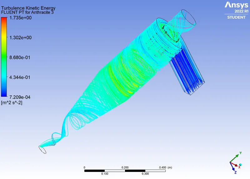
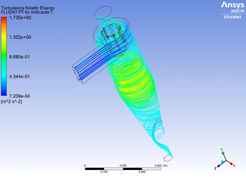
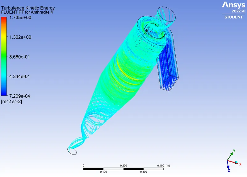
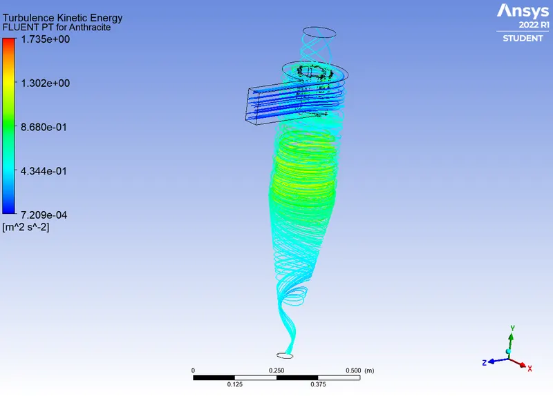
Turbulence contour:

Case 1.1 (D=1`mum`)	Case 2.1 (Vi=Vf=1m/s)
Case 1.2 (D=2`mum`)	Case 2.2 (Vi=Vf=2m/s)
Case 1.3 (D=3`mum`)	Case 2.3 (Vi=Vf=3m/s)
Case 1.4 (D=4`mum`)	Case 2.4 (Vi=Vf=4m/s)
Case 1.5 (D=5`mum`)	Case 2.5 (Vi=Vf=5m/s)

Computed values of particle and pressure data:

	Case 1.1 (D=1`mum`)	Case 1.2 (D=2`mum`)	Case 1.3 (D=3`mum`)	Case 1.4 (D=4`mum`)	Case 1.5 (D=5`mum`)
Particle tracked	378	378	378	378	378
Particle trapped	300	301	305	290	241
Particle escaped	78	77	73	87	137
Particle incomplete	0	0	0	1	0
Inlet pressure	26.175 pa	26.175 pa	26.175 pa	26.175 pa	26.175 pa
Outlet pressure	-0.011 pa	-0.011 pa	-0.011 pa	-0.011 pa	-0.011 pa

	Case 2.1 (Vi=Vf=1m/s)	Case 2.2 (Vi=Vf=2m/s)	Case 2.3 (Vi=Vf=3m/s)	Case 2.4 (Vi=Vf=4m/s)	Case 2.5 (Vi=Vf=5m/s)
Particle tracked	378	378	378	378	378
Particle trapped	312	292	241	258	291
Particle escaped	66	86	137	108	82
Particle incomplete	0	0	0	12	5
Inlet pressure	2.274 pa	11.332 pa	26.175 pa	47.71 pa	76.121 pa
Outlet pressure	-0.0006 pa	-0.0078 pa	-0.0211 pa	-0.0418 pa	-0.070 pa

Inference:

	Case 1.1 (D=1`mum`)	Case 1.2 (D=2`mum`)	Case 1.3 (D=3`mum`)	Case 1.4 (D=4`mum`)	Case 1.5 (D=5`mum`)
Efficiency	79.36%	79.62%	80.68%	76.71%	63.75%
Pressure drop	26.1868 pa	26.1868 pa	26.1868 pa	26.1868 pa	26.1868 pa

	Case 2.1 (Vi=Vf=1m/s)	Case 2.2 (Vi=Vf=2m/s)	Case 2.3 (Vi=Vf=3m/s)	Case 2.4 (Vi=Vf=4m/s)	Case 2.5 (Vi=Vf=5m/s)
Efficiency	82.53%	77.24%	63.75%	68.25%	76.98%
Pressure Drop	2.2746 pa	11.3398 pa	26.195 pa	47.75 pa	76.191 pa

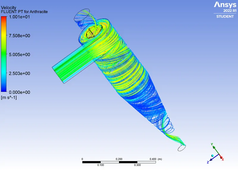
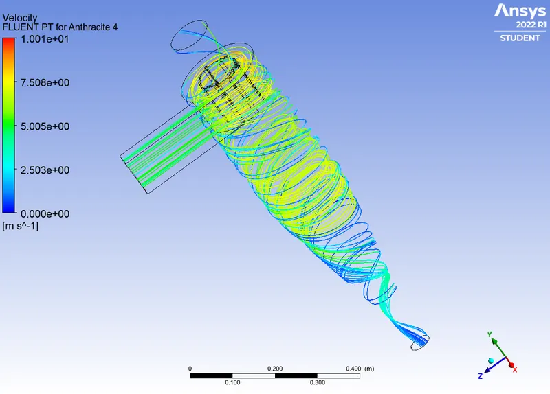
From the results, it is evident that eth efficiency of the cyclone increases with increasing particle mean diameter and density. The ideal velocity for maximum efficiency would be around 5m/s and so there is a difference in efficiency when there is a difference in velocity. The efficiency also depends on the tangential velocity, cyclone diameter, cyclone length, separator exit geometry. From the experimental results is it noted that typically increasing the gas tangential velocity, decreasing the cyclone diameter, increasing cyclone length would lead to increase in efficiency.

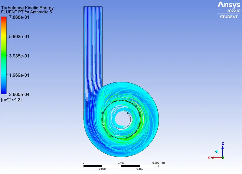
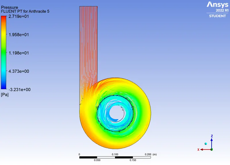
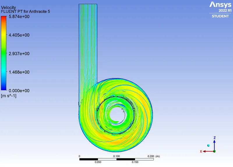
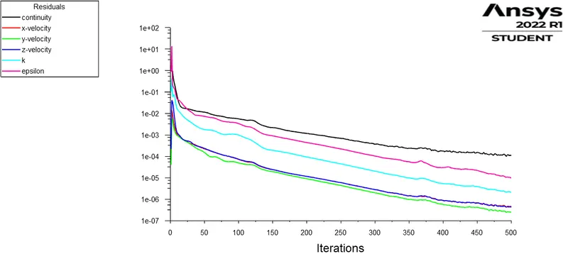
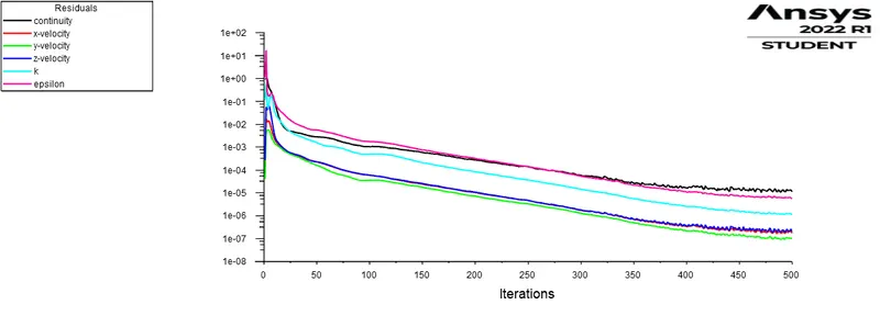
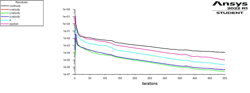
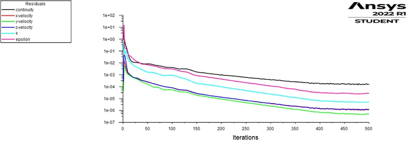
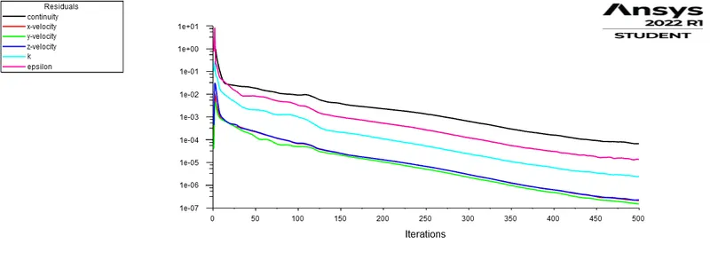
Different cases of varying diameter and varying velocity is simulated for the results to be observed. In terms of the solver efficiency, the solution appears to be converged at above 50 iterations for all the cases, and hence it is noted that the operating conditions of the cyclone are conveniently under the steady state.

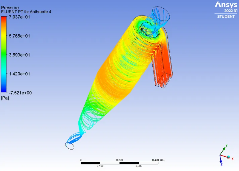
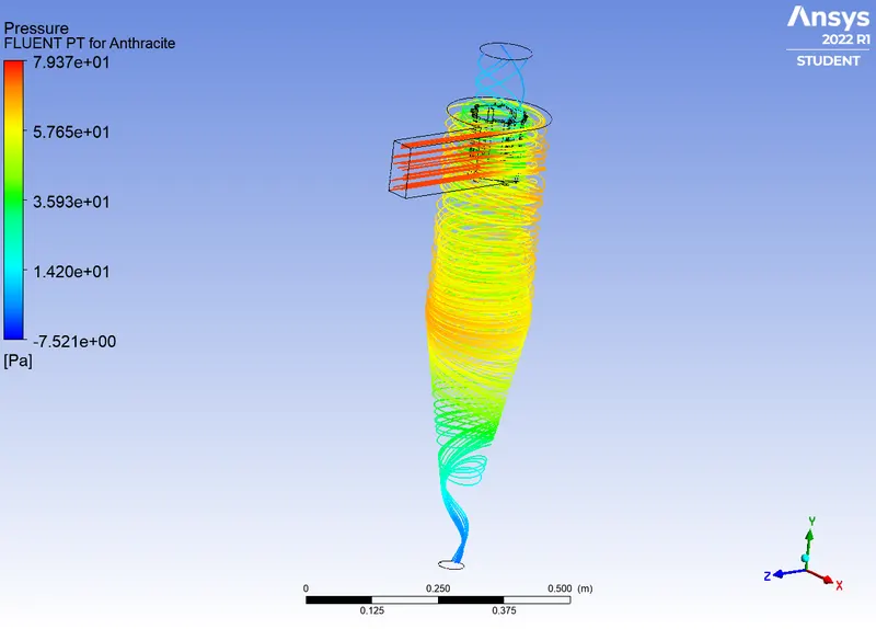
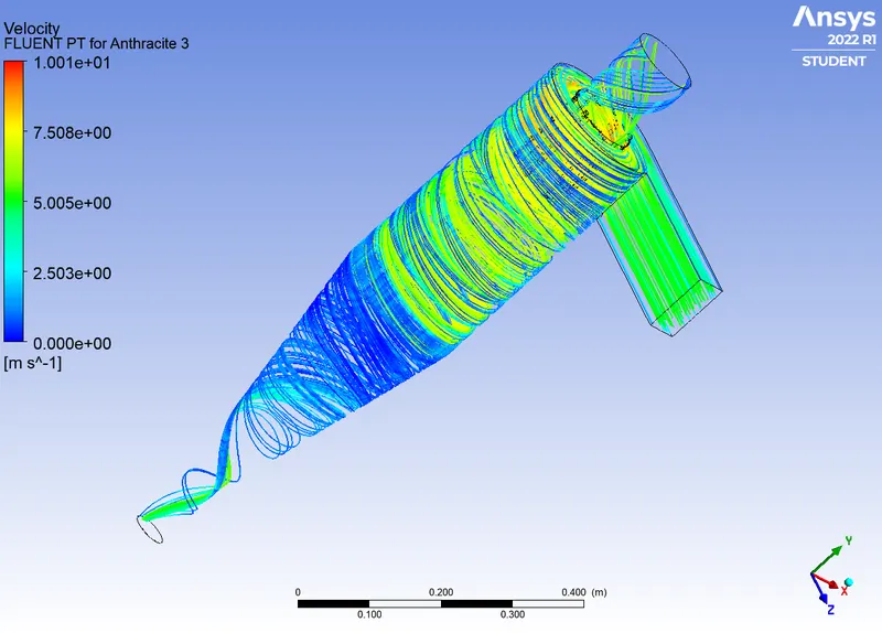
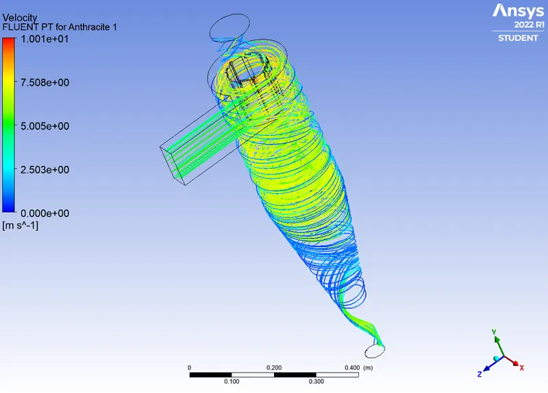
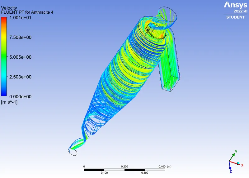
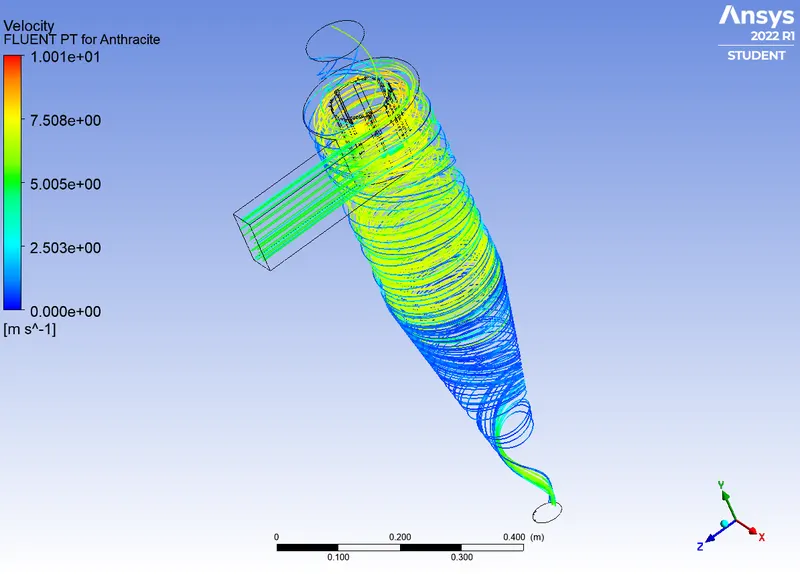
Particle size, flow velocity and inlet velocity are the physical process parameters varied here. The pressure plot clearly shows that though there is a pressure drop due various losses, the velocity of the particles adds up to the kinetic energy. It is also evident that the particle size within the range 5micrometre does not have any significant influence on the pressure and velocity of the flow. But as the particle size exceeds the critical diameter, more complications would tend to grow and lead to the efficiency difference.

The collection efficiency of cyclone depends on particle size, density, geometry and velocity. Parameters such as inlet area, gas density, composition percentage plays an important role in the efficiency. The critical diameter of particles usually found by the experimental results is kept as a constant to determine the cases needed for the simulation. Then the critical diameter is once again validated by the results from the simulation.

The geometry of the separator has a greater influence on the entrainment or escape property of the particles. The exit nozzle length on the top and the inlet size is of greater importance for the particle behaviour prediction. The slant angle and exit nozzle height at the bottom solely determines the turbulence kinetic energy of the particles.

Vortex shedding:

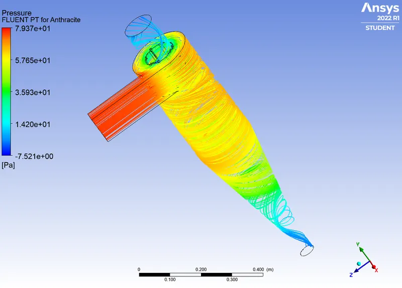
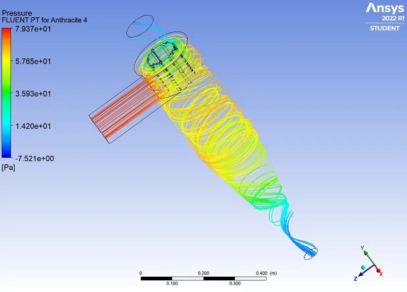
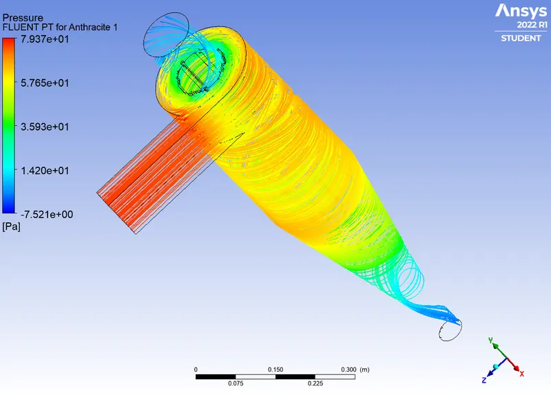
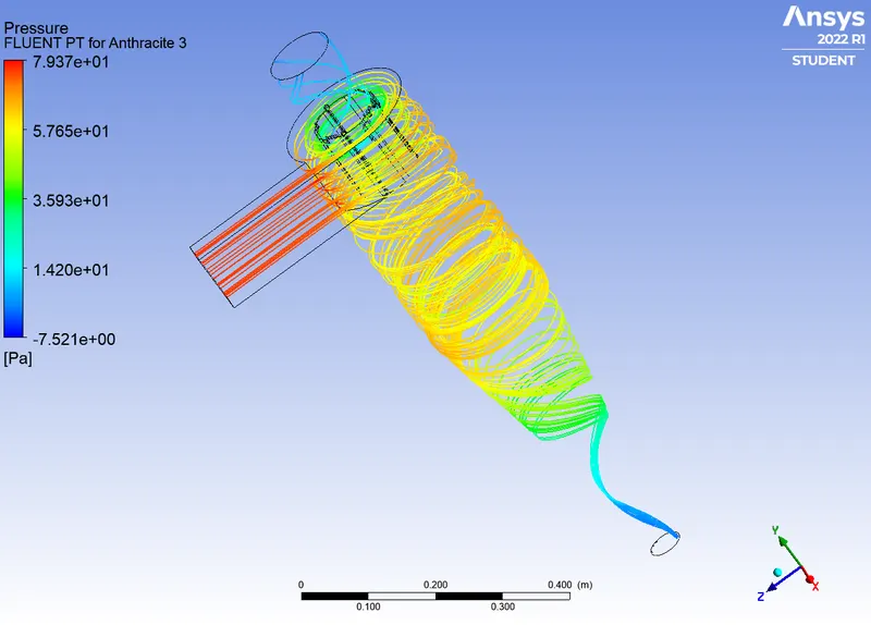
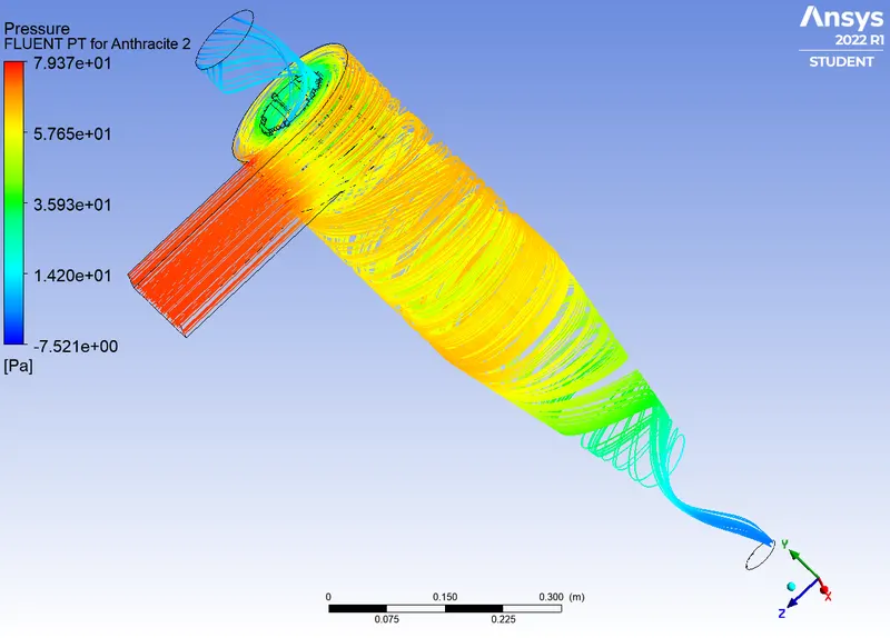
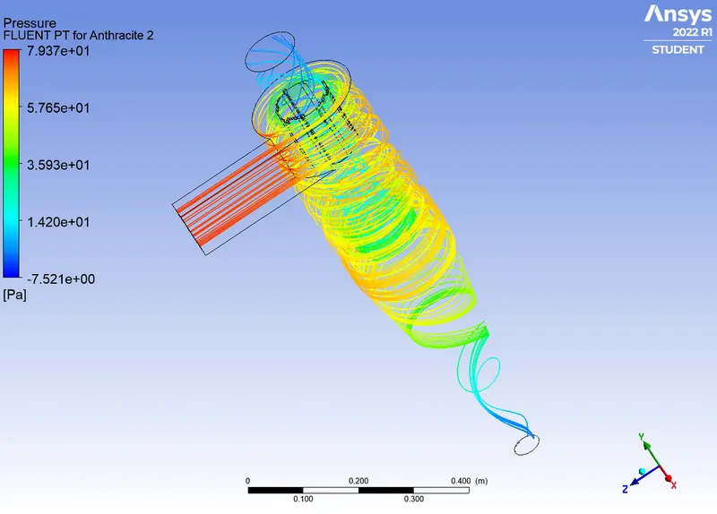
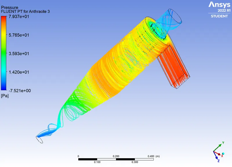
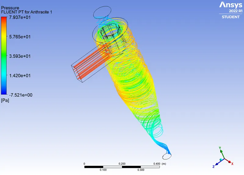
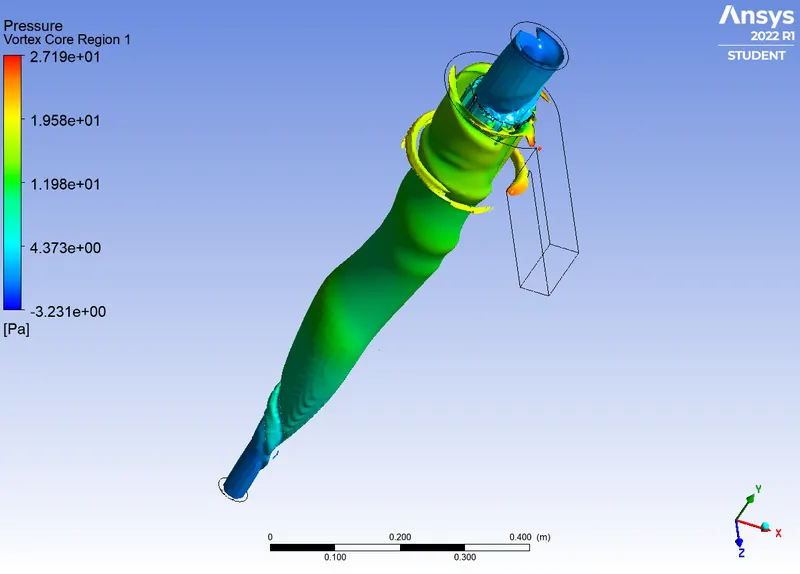
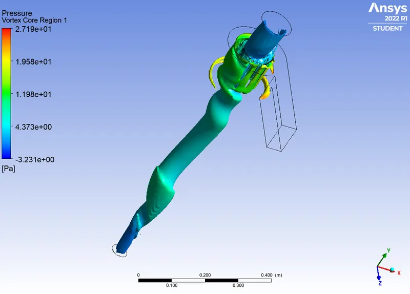
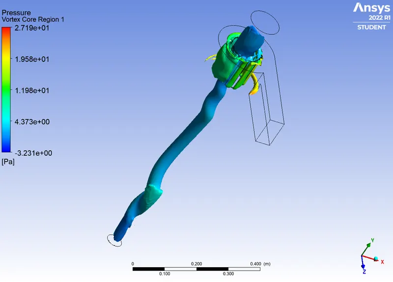
Cyclone is visually characterized by the vortex formation, and here the vortex shedding is done using the pressure drop phenomenon. The vortex with various sizes is depicted below, which explains the friction loss, energy loss, entry and exit loss in the cyclone. The swirl and energy dissipation is the most predominant cause for pressure drop. The flow velocity is a major part that leads to the growth of the vortex. It is observed that there is a higher pressure near the walls of the cyclone which forms the outer circumference. The pressure reduces when we go inner and inner towards the cyclone center of pressure.

Conclusion:

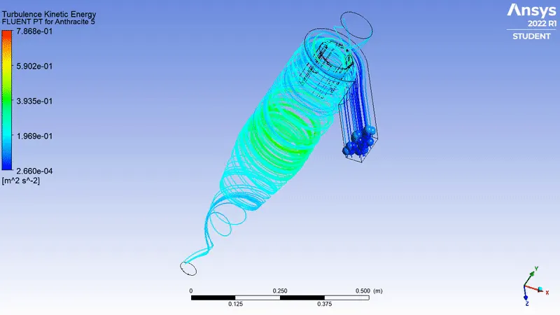
Thus the cyclone separator efficiency is calculated through simulations using Discrete phase Modelling approach. The parameters used are compared to the values computed and the observed that the geometry, flow essentials and particle property are the most concerned for efficiency calculation. On the solver efficiency the factor of DPM iteration interval should be maintained optimum and the most convenient solver should be swirl flow dominated.