Week 8 - Simulating Cyclone separator with Discrete Phase Modelling

INTRODUCTION

Many industries carries out some separation or purification stages in which process streams are separated and purified. Such separations involve physical principles based on differences in the properties of the constituents of the stream. Heterogeneous mixtures consist of components that do not react chemically and have clearly visible boundaries of separation between the different phases. Components of such mixtures can be separated using various techniques such as cyclone separator, gas-liquid separator, liquid-liquid separator, gravity separator, centrifugal separator, scrubbers, hydro-cyclone, electrostatic precipitator etc.

CYCLONE SEPARATOR

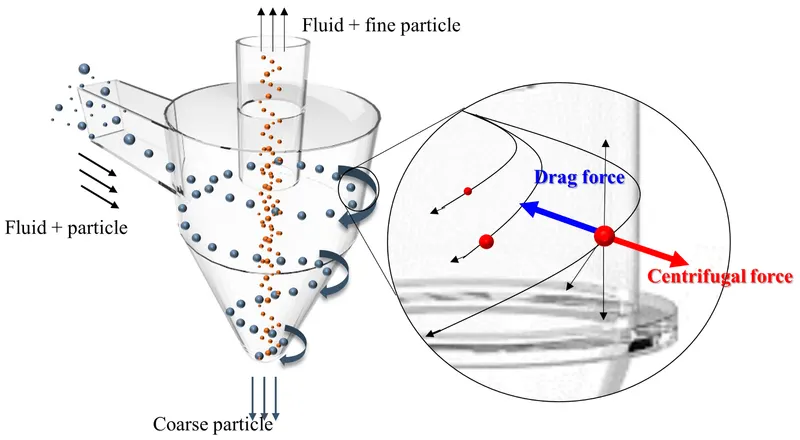
Cyclone separators provide a method of removing particulate matter from any gas stream at low cost and low maintenance. Cyclones are basically centrifugal separators, consists of an upper cylinder called as barrel and a lower conical part referred to as cone. They simply transform the inertia force of gas particle flows to a centrifugal force by means of a vortex generated in the cyclone body.

WORKING PRINCIPLE

The particle laden air stream enters tangentially at the top of the barrel and travels downward into the cone forming an outer vortex. The increasing air velocity in the outer vortex results in a centrifugal force on the particles separating them from the air stream. When the air reaches the bottom of the cone, it begins to flow radially inwards and out the top as clean air/gas while the particulates fall into the dust collection chamber attached to the bottom of the cyclone.

TYPES OF CYCLONE SEPARATOR

Cyclone separators are available in many shapes and sizes. These can range from the small 1 and 2 cm diameter source sampling cyclones which are used for particle size analysis to the large 5 m diameter cyclone separator used after wet scrubbers. According to the entry cyclone separators are classified as tangential entry and axial entry separators. The former type are widely used in power and cement plants, feed mills and other process industries. The latter is used in multi cyclone configuration as these provide higher efficiency.

EFFICIENCY OF CYCLONE SEPARATOR

The collection efficiency of cyclones varies as a function of density, particle size and cyclone design. Cyclone efficiency will generally increase with the increase in particle size and/or density, inlet duct velocity, cyclone body length, number of gas revolutions in the cyclone, ratio of cyclone diameter to gas exit diameter, inlet dust loading, and smoothness of the cyclone inner wall.

Similarly, cyclone efficiency will decrease with increase in parameters such as gas viscosity, cyclone body diameter, gas exit diameter, gas inlet duct area, gas density, leakage of air into the dust outlet etc.

Four empirical models used to calculate the cyclone efficiency are:-

IOZIA AND LEITH MODEL

Iozia and Leith model is a modified version of Barth model, which is developed based on the force balance. The model assumes that a particle carried by the vortex endures the influence of two forces: a centrifugal force Z and a flow resistance W.

The collection efficiency is calculated by: -

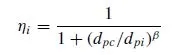
Where d_pi is the particle diameter and d_pc is the cut size diameter.

β is the expression for slope diameter derived according to the following formula: -

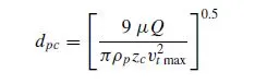
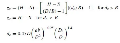
Where core length z_c and core diameter d_c are given as: -

LI AND WANG MODEL

The Li and Wang model includes particle bounce and turbulent diffusion at the cyclone wall. A two dimensional analytical expression of particle distribution in the cyclone is obtained. This model is based on following assumptions:

• The radial particle velocity and the radial concentration profile are not constant for uncollected particles within the cyclone.
• Boundary conditions with the consideration of turbulent diffusion coefficient and the particle bounce re-entrainment on the cyclone wall are:

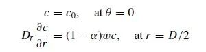
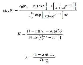
The concentration distribution in a cyclone is given as:

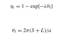
The resultant expression of the collection efficiency for particle of any size is given as

KOCH AND LICHT MODEL

Koch and Licht collection theory recognized the inherently turbulent nature of cyclones and the distribution of gas residence times within the cyclone. The assumptions made in the model were: -

• The tangential velocity of a particle is equal to the tangential velocity of the gas flow, i.e. there is no slip in the tangential direction between the particle and the gas.
• The tangential velocity is related to the radius of cyclone by: uRⁿ = constant

A force balance and an equation on the particles collection yields the grade efficiency as: -

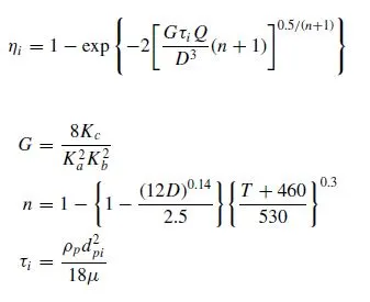
G is the factor related to the configuration of the cyclone, n is related to the vortex and τ is the relaxation term.

LAPPLE MODEL

Lapple model was developed on force balance without considering the flow resistance. Lapple assumed that a particle entering the cyclone is evenly distributed across the inlet opening. The particle that travels from inlet half width to the wall in the cyclone is collected with 50% efficiency. The semi empirical relationship developed by lapple to calculate a 50% cut diameter d_pc.

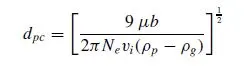
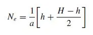
Where N_e is the number of revolutions

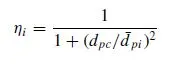
The efficiency of collection of any size of particle is given by

GEOMETRY

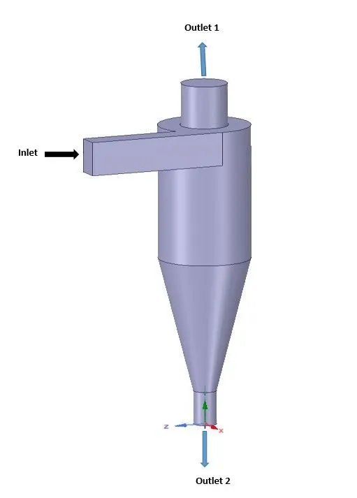
A 3D geometry of tangential entry cyclone separator has been used in the present analysis. Fluid volume has been extracted using the volume extract feature available in Spaceclaim.

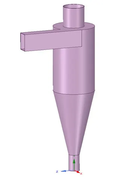
Extracted fluid volume

MESHING

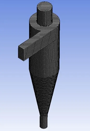
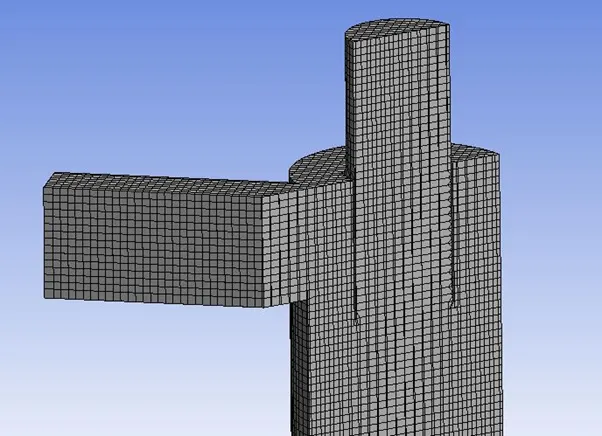
Assembly meshing technique has been used to discretize the computational domain. CutCell meshing is a general purpose hex-dominant meshing technique. The CutCell meshing algorithm is suitable for a large range of applications, and due to the large fraction of hex cells in the mesh, often produces better results than regular tetrahedral meshes.

The figure below shows the grid arrangement for the fluid volume.

Element quality: -

Max = 0.99974

Min = 0.21597

Orthogonal quality: -

Max = 1

Min = 0.23662

Skewness: -

Max = 0.9661

Min = 1.3057e-010

CASE SETUP: -

The present study investigates the cyclone separator performance for different particle sizes varying from 1µm to 5 µm and velocity of particle varying from 1m/s to 5m/s. Table 1 represents the various cases considered for evaluation of collection efficiency. As the collection efficiency of cyclone separator depends on various factors, the more dominating parameters have been reported in the present simulation.

The various settings used to set up the present case has been discussed below with relevant snippets.

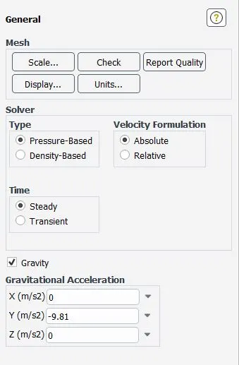
General settings

Solver: - pressure based solver

Time: - steady

Gravity: - -9.81 in y direction

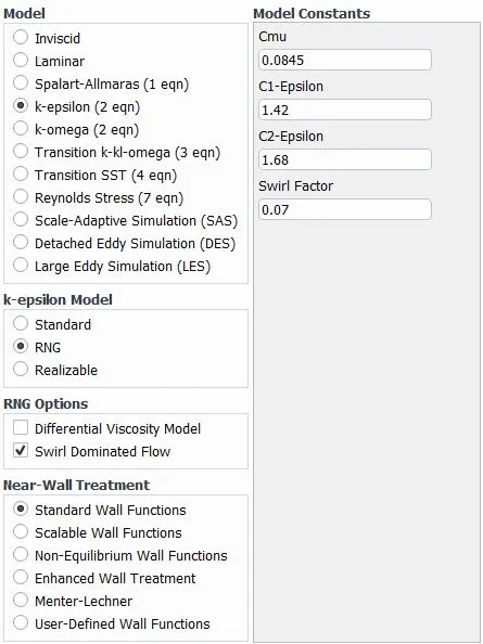
Viscous model: - RNG K-epsilon model has been used with swirl dominated flows as it provides better results for strong swirling flows typically found in cyclone separators.

Discrete phase model: -

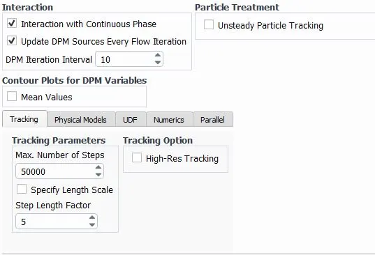
• Enabling the “interaction with continuous phase option” sets the flow as coupled flow which means the discrete particles are now affected by the continuous phase.
• Update DPM sources option enables us to capture the particles source terms at every DPM iteration interval.
• Tracking parameters is used to control the time integration of the particle trajectory equation.
• Max number of steps defines the limit on the integration time steps after which the particle trajectory is terminated and reported as incomplete.
• Step length factor also controls the time step size used to integrate the equation of motion for the particle. Larger the step length factor smaller is the time step size.
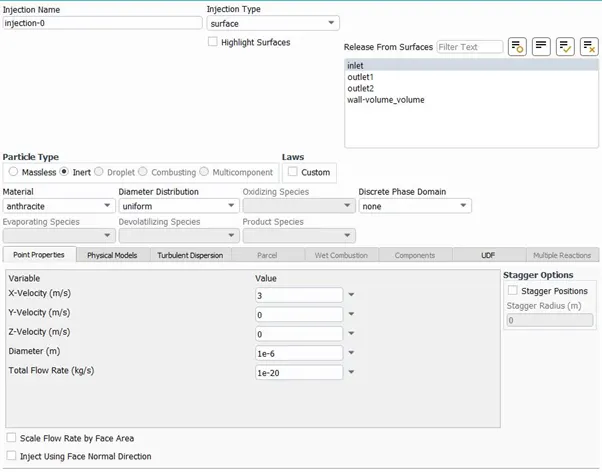
• Particle injection: -

  Particle type – inert

  Material – anthracite

  Injection type – surface

  Release from surface – inlet

  Diameter – 1e-6 to 5e-6

Boundary conditions: -

The boundary conditions are expressed as below: -

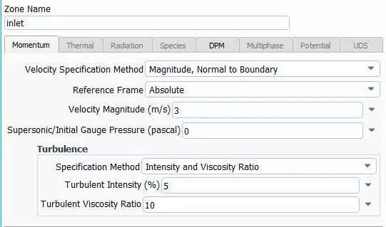
Inlet:-

Velocity = 3m/s

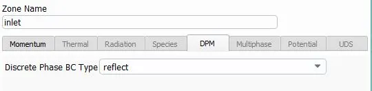
Discrete phase BC type – reflect

Outlet: - (pressure outlet)

Outlet 1 - Discrete phase BC type – escape

Outlet 2 - Discrete phase BC type – trap

Wall: -

Discrete phase BC type – reflect

Reflect - the particle rebounds off the boundary in question with a change in its momentum as defined by the coefficient of restitution.

Trap – the trajectory calculations are terminated and the fate of the particle is recorded as trapped.

Escape – the particle is reported as having escaped when it encounters the boundary in question. Trajectory calculations are terminated.

Solution methods: -

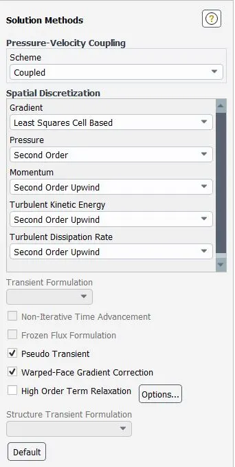
Pressure velocity coupling scheme – coupled scheme

Pressure, momentum, turbulent kinetic energy and turbulent dissipation rate have been discretized using second order upwind scheme for more accurate results.

RESULT AND DISCUSSION

In this section separation efficiency has been calculated for various particle diameter ranging from 1µm to 5µm and in another case velocity has been varied keeping the particle diameter fixed.

SEPARATION EFFICIENCY

The separation or collection efficiency is a measurement of a cyclone’s ability to separate particles from the flowing gas stream. In the present simulation, according to the particle history data separation efficiency can be calculated as the ratio of number of particles trapped to the number of particles tracked.

PRESSURE DROP

The pressure drop across the cyclone significantly affects the performance parameters of a cyclone. The total pressure drop in a cyclone is due to the entry and exit losses, and friction and kinetic energy losses in the cyclone. Swirl and energy dissipation is also a major cause of pressure drop.

Pressure drop can be calculated as: -

Total pressure drop = total inlet pressure – total outlet pressure

Case 1

Particle size = 1µm, velocity = 3m/s

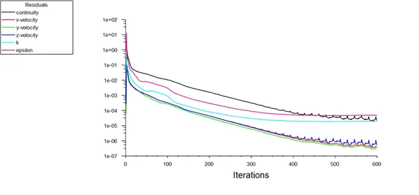
Residual plot

Particle resident time

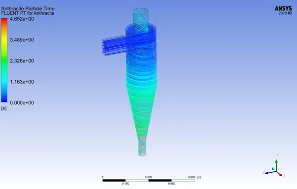
Particle tracking

Separation efficiency = (17/120)*100

= 14.16 %

Case 2

Particle size = 2µm, velocity = 3m/s

Residual plot

Particle resident time

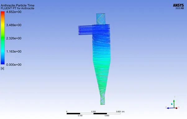
Particle tracking

Separation efficiency = (47/120)*100

= 39.16 %

Case 3

Particle size = 3µm, velocity = 3m/s

Residual plot

Particle resident time

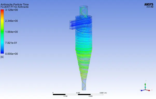
Particle tracking

Separation efficiency = (96/120)*100

= 80 %

Case 4

Particle size = 4µm, velocity = 3m/s

Residual plot

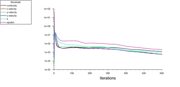
Particle resident time

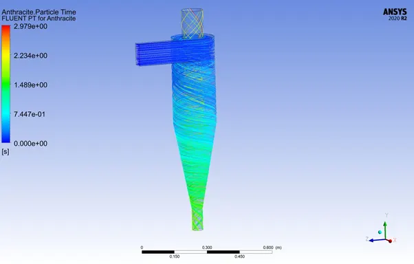
Particle tracking

Separation efficiency = (106/120)*100

= 88.34 %

Case 5

Particle size = 5µm, velocity = 3m/s

Residual plot

Particle resident time

Particle tracking

Separation efficiency = (118/120)*100

= 98.34 %

Pressure drop

Since the velocity is same for all the cases the pressure drop in all the cases is same.

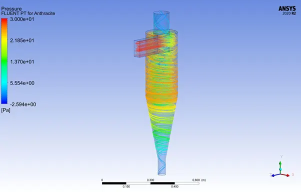
Total inlet pressure = 29.072149 pa

Total outlet pressure = 0.02050 pa

Total pressure drop = (29.072149 – 0.02050)

= 29.05 pa

Pressure contour

Case 6

Particle size = 5µm, velocity = 1m/s

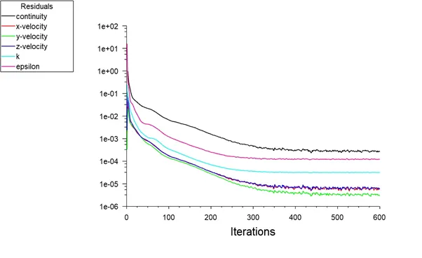
Residual plot

Particle resident time

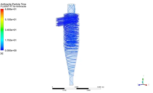
Particle tracking

Separation efficiency = (1/162)*100

= 0.61 %

Pressure drop = inlet pressure – outlet pressure

= 2.292 – 0.000315

= 2.291 pa

Case 7

Particle size = 5µm, velocity = 2m/s

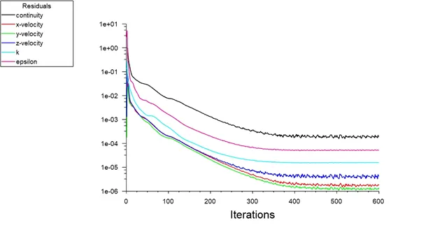
Residual plot

Particle resident time

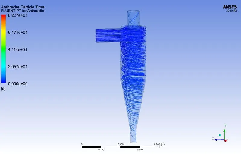
Particle tracking

Separation efficiency = (101/162)*100

= 62.34 %

Pressure drop = 10.813 - 0.0035

= 10.80 pa

Case 8

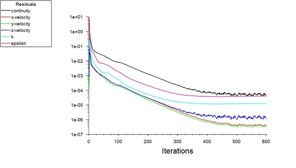
Particle size = 5µm, velocity = 3m/s

Residual plot

Particle resident time

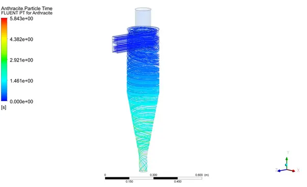
Particle tracking

Separation efficiency = (156/162)*100

= 96.29 %

Pressure drop = 25.268 – 0.0098

= 25.25 pa

Case 9

Particle size = 5µm, velocity = 4m/s

Residual plot

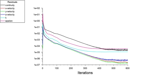
Particle resident time

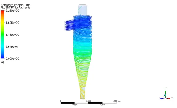
Particle tracking

Separation efficiency = (160/162)*100

= 98.76 %

Pressure drop = 45.9864 – 0.0206

= 45.965 pa

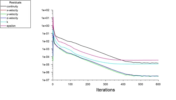
Case 10

Particle size = 5µm, velocity = 5m/s

Residual plot

Particle resident time

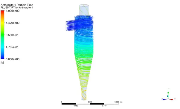
Particle tracking

Separation efficiency = (156/162)*100

= 96.29 %

Pressure drop = 73.08325 – 0.0366

= 73.046 pa

swirling strength

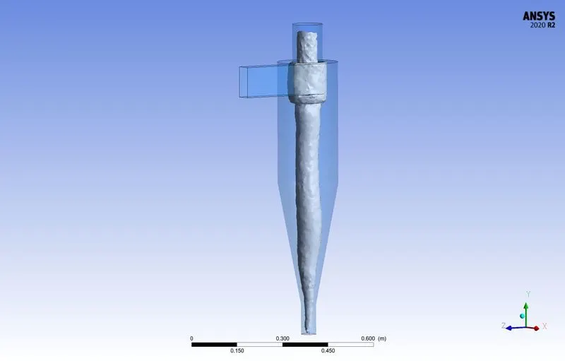
vorticity

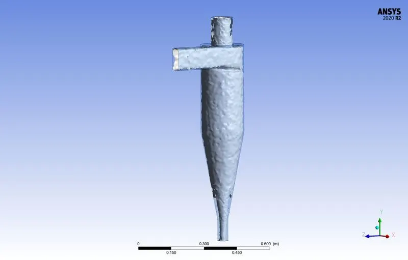
Table 1: Different case of particle diameter and velocity considered in present simulation

Cases	Particle dia (m)	Velocity (m/s)	Particle tracked	Particle trapped	Separation efficiency (%)	Pressure drop (pa)
1	1.00E-06	3	120	17	14.16	29.05
2	2.00E-06	3	120	47	39.16
3	3.00E-06	3	120	96	80
4	4.00E-06	3	120	106	88.341
5	5.00E-06	3	120	118	98.34
6	5.00E-06	1	162	1	0.61	2.29
7	5.00E-06	2	162	101	62.34	10.80
8	5.00E-06	3	162	156	96.29	25.25
9	5.00E-06	4	162	160	98.76	45.965
10	5.00E-06	5	162	156	96.29	73.04

Effect of particle diameter on separation efficiency

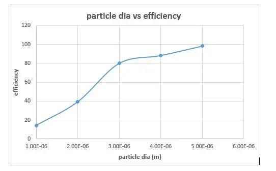
From the graph it can be observed that separation efficiency gradually increases with increase in particle diameter. Larger particles can be easily separated as compared to the smaller particles. Particles smaller than 5 microns are difficult to separate without using very small separator. To extract very fine particles from the gas stream a small diameter cone can be used.

Effect of particle velocity on separation efficiency

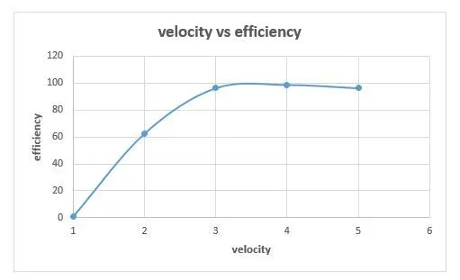
The plot between particle inlet velocity and separation efficiency clearly shows that there is rapid increase in separation efficiency with small increment in velocity. Higher velocity results in higher pressure drop and it can be concluded that high efficiency cyclones are likely to have the highest pressure drop.

Excessive increasing of the velocity of particles is also not beneficial as it leads to high level of erosion if the gas stream contains abrasive particles.

Conclusions

• The maximum efficiency obtained is around 98.78 % and is achieved for the case of particle diameter 5µm and velocity of 4m/s.
• The efficiency increases with increase in particle diameter.
• The efficiency increases with increment in particle velocity.
• High efficiency cyclones have higher pressure drop.