Conjugate Heat Transfer Analysis on a graphics card.

AIM: - To perform conjugate heat transfer simulation on graphics card.

OBJECTIVES:-

1) To learn about conjugate heat transfer analysis in Ansys fluent.

2) To learn meshing concepts for more accurate results.

INTRODUCTION

CONJUGATE HEAT TRANSFER ANALYSIS

Conjugate heat transfer analysis is done to study the thermal interaction between solids and fluids, which is caused due to temperature differences between solids and fluids. In solids conduction is the mode of heat transfer and convection in fluids. In CHT analysis multiregion mesh is created to have a clear definition of the interfaces in the computational domain.

CHT analysis are carried out for some of the typical problems such as:-

• Heat Exchangers
• Cooling of electronic equipment
• HVAC systems
• Overall heat transfer coefficient, e.g. for a car radiator.
• Highest (or lowest) temperature in a system, e.g. in a gas turbine, chemical reaction vessels, food ovens.
• Temperature distribution (related to thermal stress), e.g. in the walls of a spacecraft.
• Temperature response in time dependent heating/cooling problems, e.g. engine cooling

3D GEOMETRY

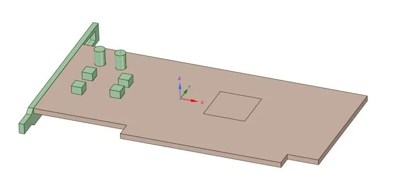
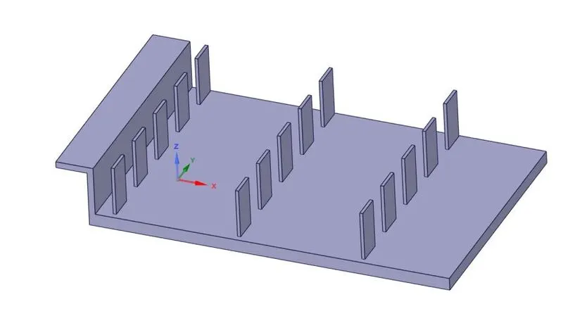
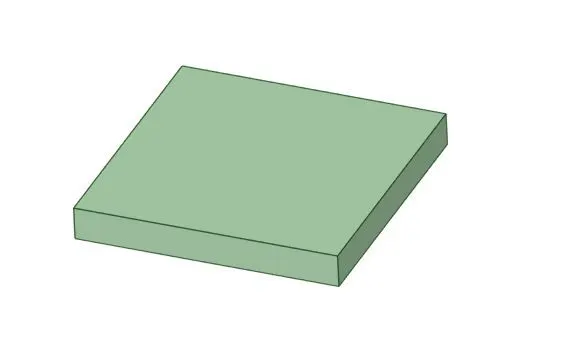
The geometry consists of graphics card and air enclosure around it. The figure below shows the graphics card and its individual components.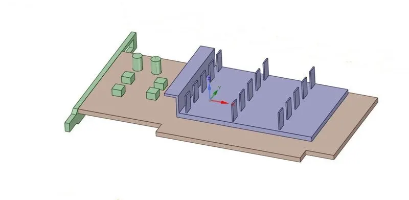

Base	Fins	Processor

Materials and their properties

	Material	Density (kg/m3)	Sp. Heat (J/kg K)	Thermal conductivity (W/mK)
Fins	Aluminium	2719	871	202.4
Processor	Silicon	2000	710	150
PCB	FR4	1850	950	0.29
Fluid	Air	1.225	1006.43	0.0242

CFD INVESTIGATION METHOD

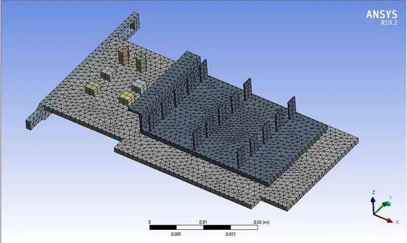
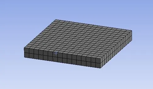
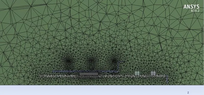
The CHT analysis has been conducted for two mesh configuration. The base mesh has been generated and then it has been refined at areas near processor to accurately calculate the maximum temperature and heat transfer coefficient of the processor. The simulation has been carried out for three different air velocities ranging between 1 m/s to 5 m/s.

CASE 1:- Base mesh

Element sizes:

processor = 0.5 mm

fins = 1mm

base = 1mm

enclosure:- min = 1mm , max = 2mm

No. of elements = 364758

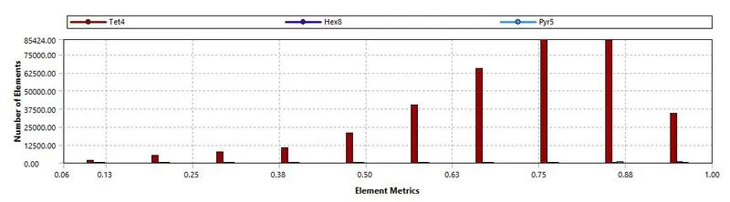
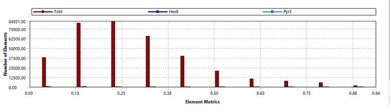
mesh quality:-

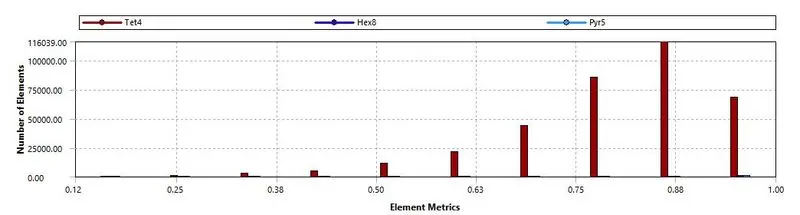
Orthogonality

Skewness

CASE SETUP :-

solver - Pressure based solver

Turbulance model - K-ε realizable model

pressure velocity coupling - SIMPLE algorithm

boundary conditions:-

inlet velocity = 1m/s

heat generation rate = 2.343e7 w/m^3

RESULT AND DISCUSSIONS

Residuals

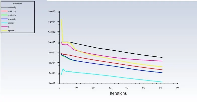
The solution got converged at 61 iterations.

Temperature contour plot

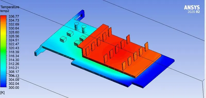
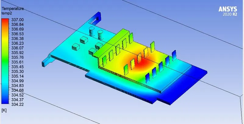
From the tempearture contour plot it is observed that the maximum temperature attained by the processor is 64 deg C. The fins helps in dissipating the heat from the processor as it increases the surface area with which the air comes into contact.

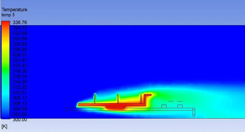
Temperature on y plane

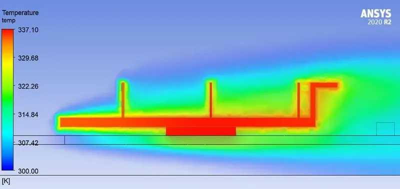
temperature volume rendering

Processor temperature

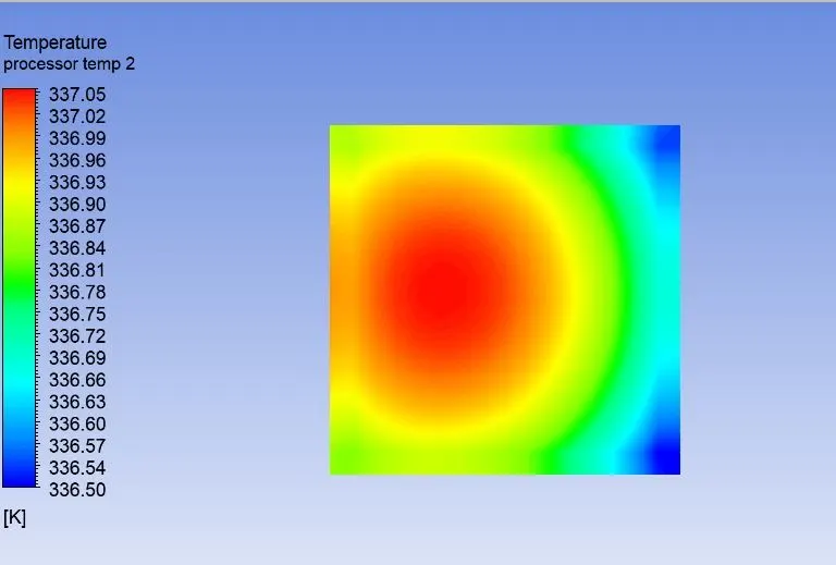
The Temperature contour shows that the hotspot is generated just behind the center as the air which comes into contact with the front edges reduces the temperature.

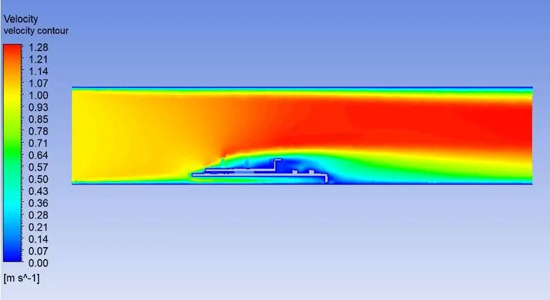
velocity contour

Velocity vector

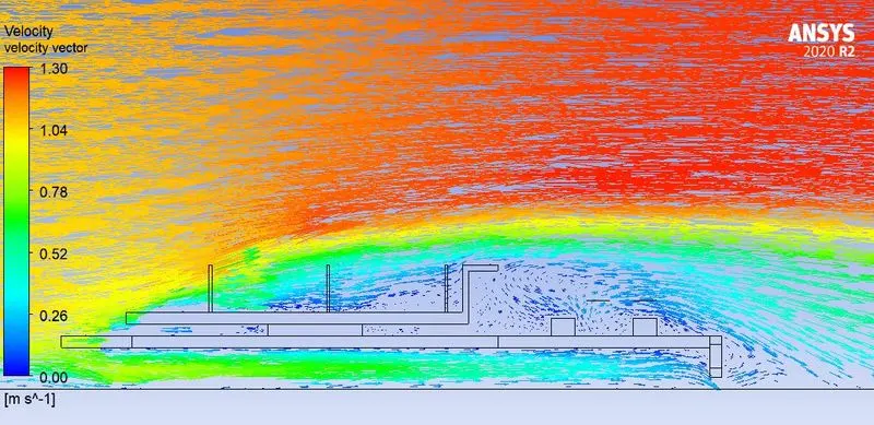
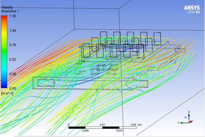
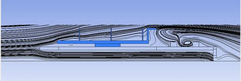
from the velocity vector it can be clearly observed that there are recirculation zones being formed just behind the fins base. these recirculation zones are areas of low velocity which reduces the heat transfer. To have a good heat transfer between graphics card and air these recircualtion zones have to be reduced. These recircualtion zones can be vizualised using velocity streamlines.

Velocity streamlines

recirculation zones

Heat transfer coefficient

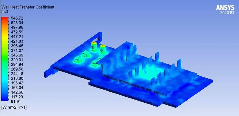
The heat transfer coefficient contour shows the average heat transfer coefficient value around 438.285 W/m^2 K.

It can also be observed that the contour is not so smooth, which signifies that refining the mesh near processor could give us more accurate values of heat transfer coefficiecnt and maximum temperature.

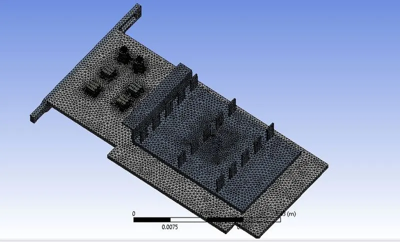
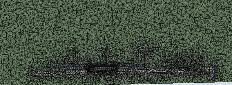
CASE 2:- Fine mesh

Element sizes:

processor = 0.2 mm

fins = 0.6mm

base = 0.8mm

enclosure:- min = 1mm , max = 1.5mm

No. of elements = 922801

Element quality

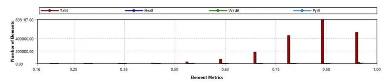
min quality = 0.15913 , max quality = 0.99994

Orthogonal quality

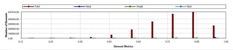
min = 0.12087 , max = 1

Skewness

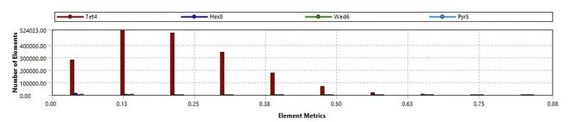
min = 9.9913e-006 , max = 0.87913

CASE SETUP :-

solver - Pressure based solver

Turbulance model - K-ε realizable model

pressure velocity coupling - SIMPLE algorithm

boundary conditions:-

inlet velocity = 1m/s , 2.5m/s , 5m/s

heat generation rate = 2.343e7 w/m^3

RESULT AND DISCUSSIONS

Residuals

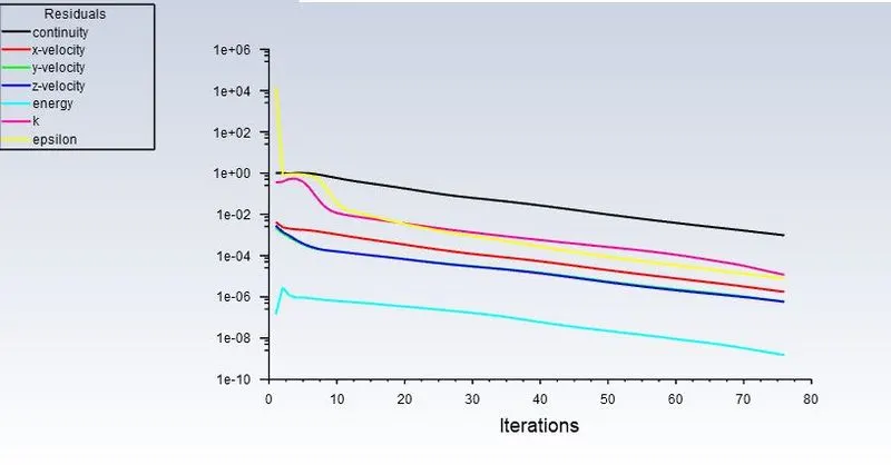
The solution got converged at 78 iterations.

Temperature contour plot

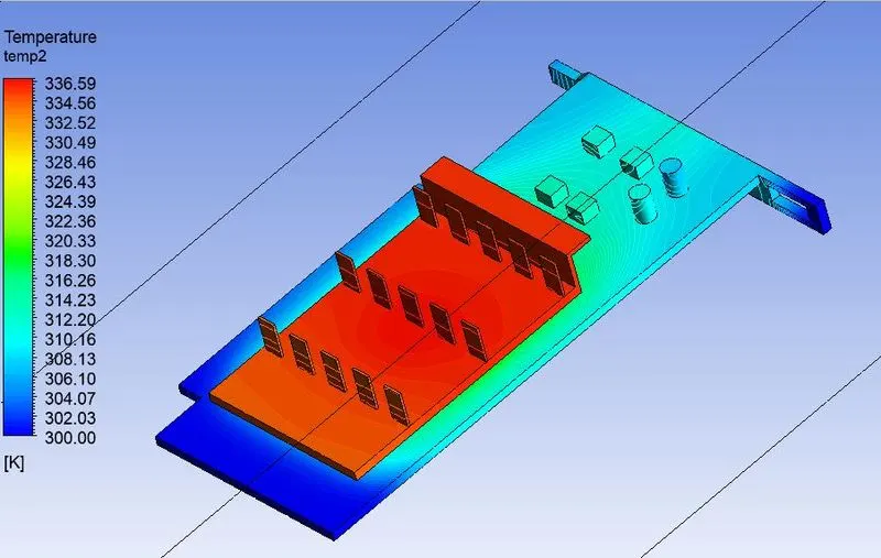
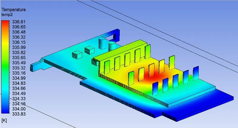
After refining the mesh the maximum temperature of the graphics card is observed to be 63 deg celcius.

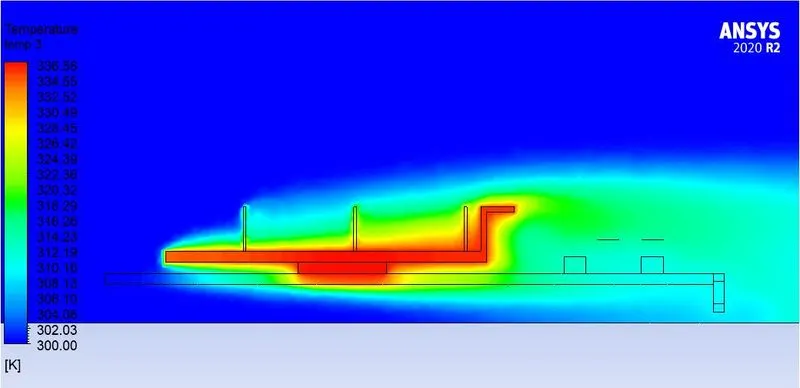
temperature on y plane

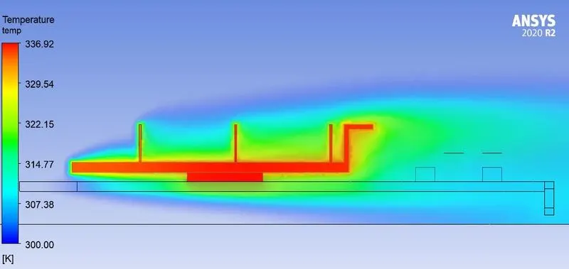
temrperature volume rendering

Processor temperature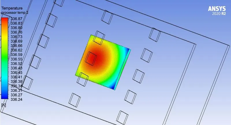

velocity contour plot

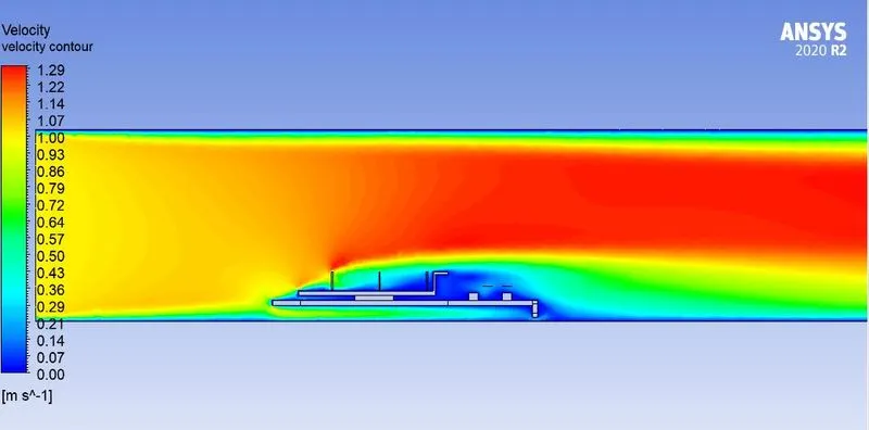
velocity vector

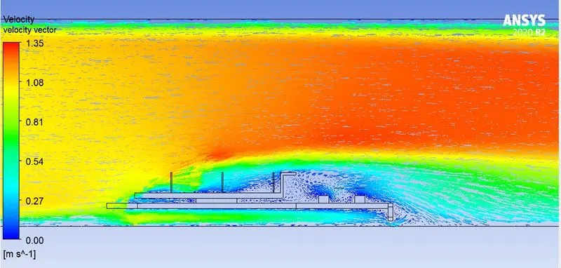
streamlines

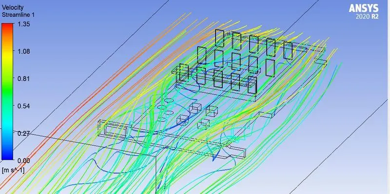
recirculation zones

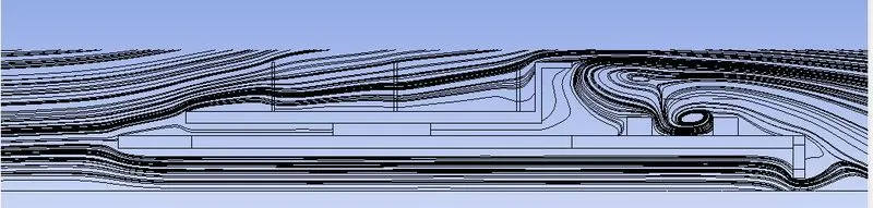
with the refinement of mesh we can clearly visualise the two recircultion zones being formed just behind the fins base.

heat transfer coefficient

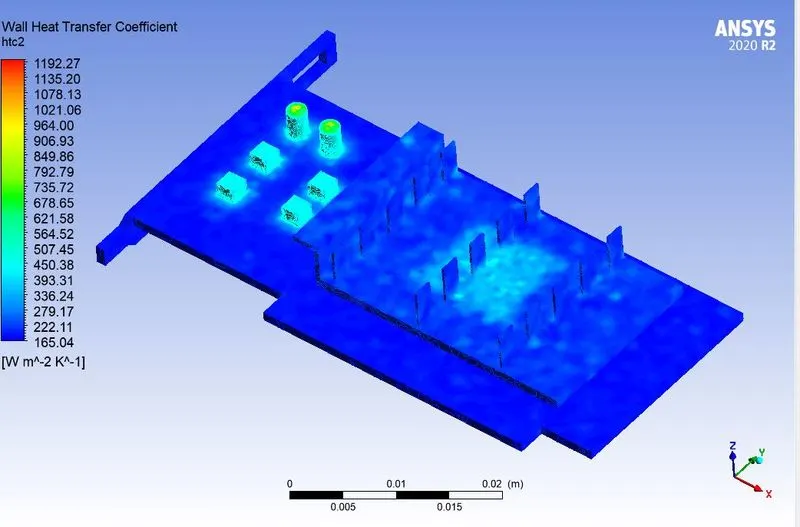
The following table represents the variation of maximum temperature and heat transfer coefficient of processor with the varying air velocity.

CASE	V (m/s)	Max temp (K)	Heat transfer coefficient (W/m2 K)
Base mesh	1	337.0674	438.2854
Fine mesh	1	336.8837	441.2178
	2.5	321.0449	657.7189
	5	314.2481	835.3467

Conclusions:-

The following conclusions can be drawn from the above simulation

1) The refinement of mesh results in accurate results.

2) With the increment in velocity the maixmum temperature of the processor reduces.

3) The heat transfer coefficient is observed to increase with increment of air velocity.

4) The recirculation zones also get prominent as velocity increases, hence the fins has to be designed in such a way that it can dissipate more heat without creating such recirculation zones.