Week 8: Proportional Valve simulation

PROPORTIONATE VALVE SIMULATION:

Aim: To carry out a simulation of air flow inside a Proportionate Valve using Converge 3.0 CFD program and then post-process the results on Paraview.

Introduction: We need to observe the parameters of Air as a medium flowing inside a Proportionate valve. In this simulation we can examine the effects of various lifts of the valve on the valve.

The Transient flow simulation is used with a special feature of Fluid-Surface Interaction along with a pressure profile for input and the results are noted.

The other parameters to be observed are change in the velocity, pressure, mass flow rate through-out the flow and total cell count.

We used three different pressure ratios to run the simulation, which are as below:

• Case 1: Valve Lift = 3 mm; AMR = No; Steady State Simulation
• Case 2: Valve Lift = 4 mm; AMR = No; Steady State Simulation
• Case 3: Valve Lift = 5 mm; AMR = No; Steady State Simulation
• Case 4: Valve Lift = 3 mm; AMR = Yes; Steady State Simulation
• Case 5: Valve Lift = 4 mm; AMR = Yes; Steady State Simulation
• Case 6: Valve Lift = 5 mm; AMR = Yes; Steady State Simulation
• Case 7: Valve Lift = 3 mm; AMR = No; FSI = Yes; Transient Flow Simulation

Geometry:

- In the Converge Studio first we import the ‘STL’ file of the geometry.

- Then, we carry out a ‘Diagnosis’ on the shape created to check for any errors. If there is no error then the geometry is correct.

- Then we move to case set up.

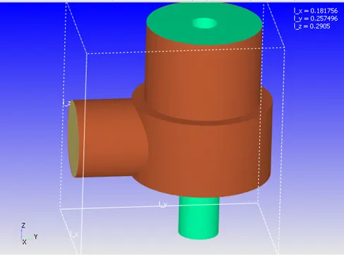
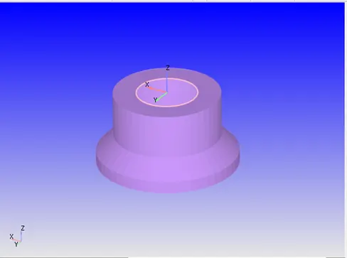
Case Set up Procedure: For Case 1, 2, 3, 4, 5, 6 - With / Without AMR [ Steady State Simulations ]

- Application Type: Time-based

- Material: Predefined Mixture = Air

- Select Gas Simulation & Reaction Mechanism.

- Reaction Mechanism: Gas Species O₂ & N₂ are the available species in the air.

- Simulation Parameters:

- Run Parameter: Steady State Solver used to perform with Full Hydrodynamic mode.

-Misc.Setting = Steady State Monitor Turned ON.

- Steady State Monitor:

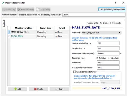
- Simulation Time Parameter:

- Start Time = 0 s

- End Time = 15000 cycles

- Initial Time Step = 1e-9 s

- Minimum Time Step = 1e-9 s

- Maximum Time Step = 1 s

- Maximum Convection CFL limit = 1.

- Solver Parameters:

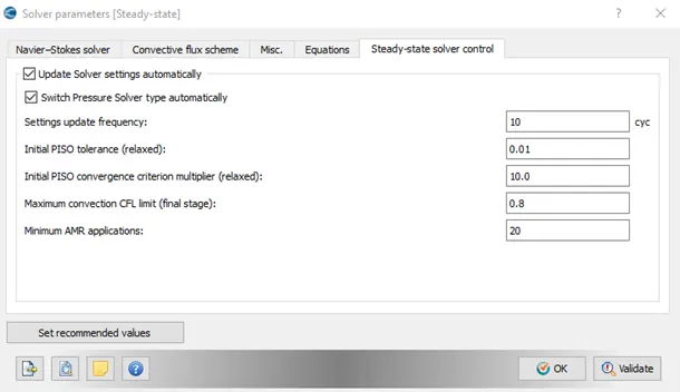
- Navier-Stokes Solver Type = ‘Density based’ selected.

- Misc. Setting:

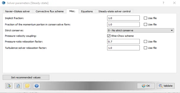
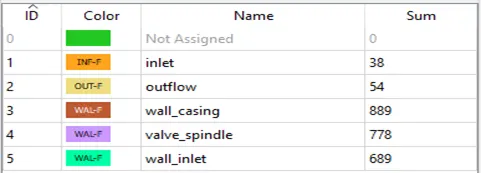
- Boundary Conditions:

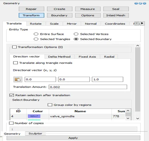
- Valve Lift Setting:

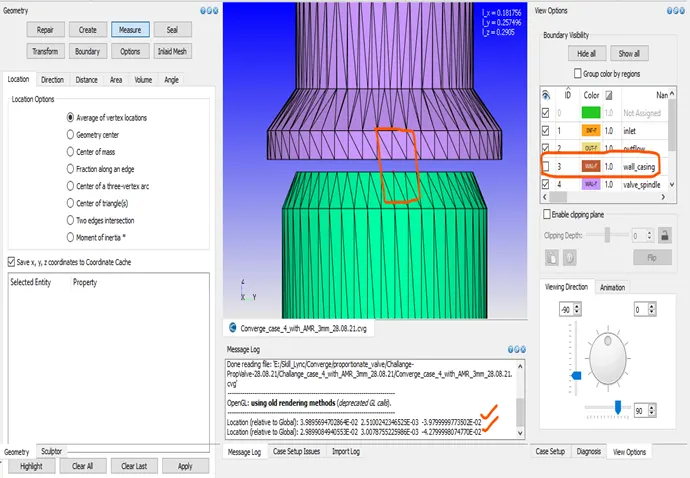
- Valve Lift Measurement: Lift = 3 mm Shown.

- Inlet Boundary Condition:

Inlet Pressure = 3000000 Pa.

Temperature = 300 K

Species: O₂ = 0.23; N₂ = 0.77 (Mass Fraction).

- Outlet Boundary Condition:

Inlet Pressure = 101325 Pa.

Temperature = 300 K

Species: O₂ = 0.23; N₂ = 0.77 (Mass Fraction).

- Wall Casing Boundary condition: Wall Motion = Stationary with Law of the Wall Condition.

- Wall Inlet Boundary condition: Wall Motion = Stationary with Law of the Wall Condition.

- Valve-Spindle Boundary Condition: Wall Motion = Stationary with Law of the Wall Condition.

- Initial Conditions & Events:

- Regions: All boundaries defined to ‘Region 0’.

Initial Pressure = set to 101325 Pa; Temp. = 300 K.

- Species Mass Fraction: O₂ = 0.23; N₂ = 0.77

- Physical Models:

- Turbulence Modelling= set to RANS [RNG K-Ɛ]

- Grid Control: For All Cases 1, 2, 3, 4, 5, 6

Base Grid Size: dx = dy = dz = 0.005 m

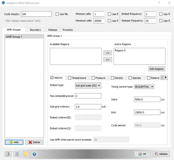
- Adaptive Mesh Refinement: For Cases 4, 5, 6 Only

- Post Processing:

- Post variables Selection:

- Typical Variables/Geometry: Select desired variables such as Density, Velocity, pressure, temperature.

- Combustion / Turbulence: Select Turbulent Kinetic Energy (tke).

- Output Files:

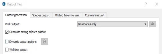
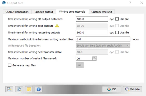
Case setup is complete for the cases 1, 2, 3, 4, 5, 6 for Steady State Simulation cases.

Case Set up Procedure: For Case 7 - - - With FSI [ Transient Flow Simulation ]

- Simulation Parameters:

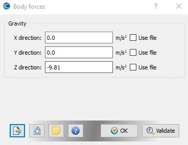
- Body Force Activation:

- Boundary Conditions:

- Inlet Boundary Condition: Inlet Pressure = Pressure Profile Setup & Species Boundary Condition = O₂ = 0.23; N₂ = 0.77 (Mass Fraction).

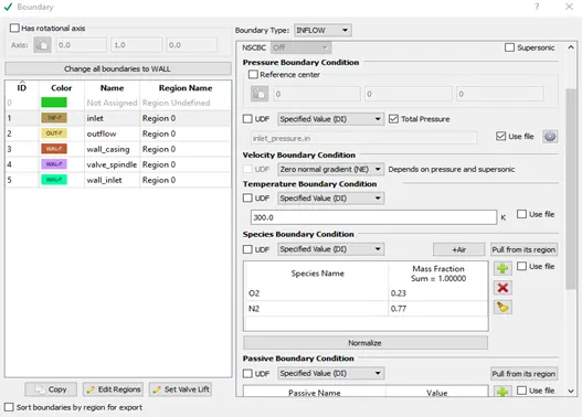
- Inlet Pressure Profile: Used a file to setup Inlet pressure profile.

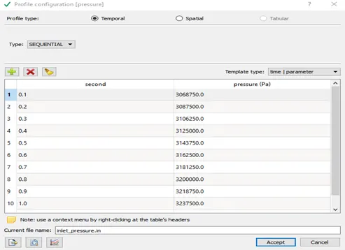
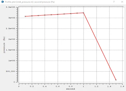
- Inlet Pressure Graph:

- Outlet Boundary Condition: Pressure = 101325 Pa; Temp. = 300 K.

- Wall Casing Boundary condition: Law of the Wall.

- Wall Inlet Boundary condition: Law of the Wall.

- Valve-Spindle Boundary Condition: Wall with “FSI”.

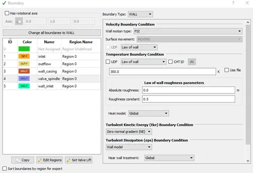
- Physical Models:

- Fluid-Structure Interaction (FSI) selected:

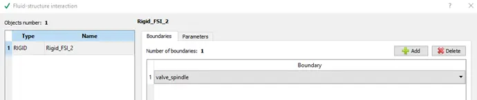
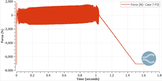
• FSI: Parameters – Force / Moments setup: Constant Applied Force = -7126 N.
• Mass Flag: Mass Value of Spindle = 3.1 Kg.

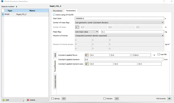
FSI: Parameters – Constrained Motion setup: 1DOF Translation with ‘Z’ direction.

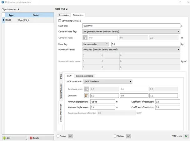
- Grid Control:

Base Grid Size: dx = dy = dz = 0.008m

- Post Processing:

- Post variables Selection:

- Typical Variables/Geometry: Select desired variables such as Density, Velocity, pressure, temperature.

- Combustion / Turbulence: Select Turbulent Kinetic Energy (tke).

- Output Files:

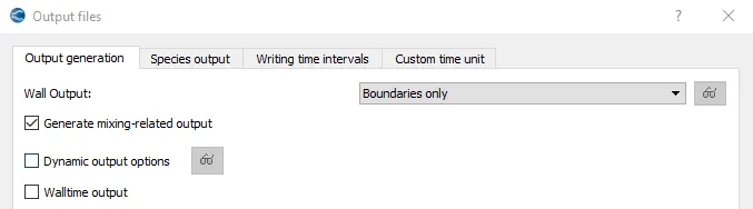
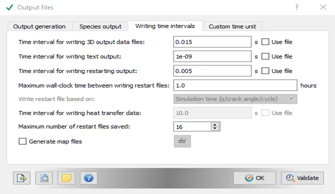
- Export case setup: The case setup files are then ‘Exported’ to the destination folders to save the details.

- The destination folders should consist of following files in order to run the simulation and then post process the result on Paraview. The files are:

(i) converge.exe (name changed for the ease of run command on cygwin)

(ii) mpiexec.exe (name changed for the ease of run command on cygwin)

(iii) post_convert.exe (under output folder)

- Open Cygwin: Now the simulation is run using Cygwin. We navigate to the desired folder where the setup files were exported.

- Command to Run Simulation: The command to run simulation through Cygwin for Converge Studio 3.0 version is as below:

“ mpiexec.exe –n 2 converge.exe restricted “

• The simulation starts running, due to which output files are generated under a separate output folder.
• These output files are then post processed to convert the data in a format suitable for Paraview.

• Inline Plot: In the Converge Studio program, we can use Inline Plotting option to plot the curves during simulation run. We can observe the change in the plots and see the position of the simulation at the end of the time.

- Post Convert in Converge: To post process, we use file type as ‘Paraview VTK in-line binary format’. Now the files are post processed with a case name ‘test’.

• This generates ‘test.vtm’ group files which are generally used in Paraview to observe the results.

- Paraview: Open Paraview to check for the results.

Observations for Cases 1,2,3,4,5,6 [ Steady State Simulations ]:

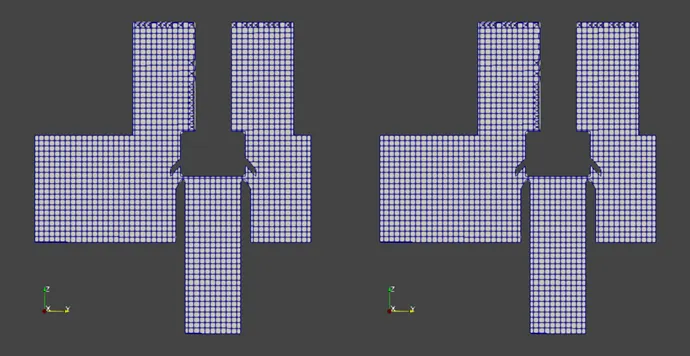
Mesh Formation: Lift = 3 mm; With & Without AMR

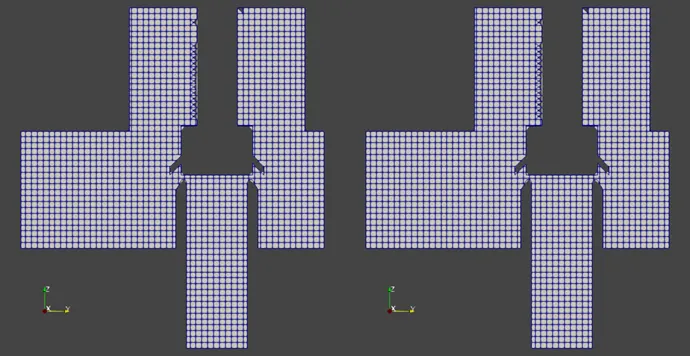
Mesh Formation: Lift = 4 mm; With & Without AMR

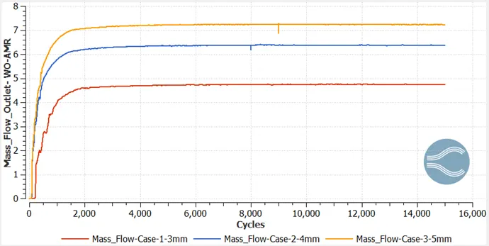
Mass Flow Rate Plot:

Without AMR:

With AMR:

Velocity Plot:

Without AMR:

With AMR:

Pressure Plot:

Without AMR:

With AMR:

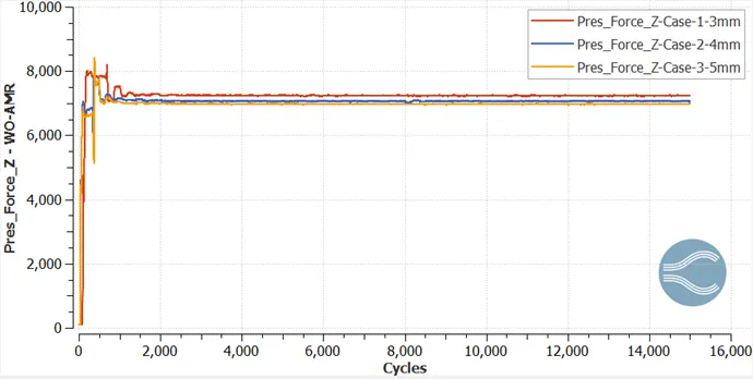
Pressure Force Plot:

Without AMR:

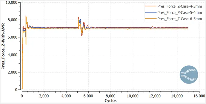
With AMR:

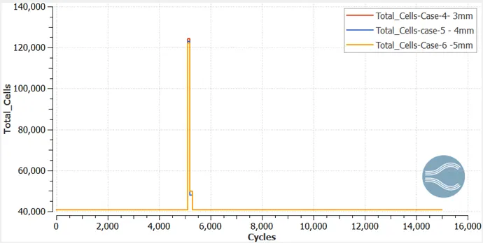
Total Cell Count: For Case 4, 5, 6 with AMR:

Pressure – Velocity Contour: Case-4 – 3 mm Lift – With AMR

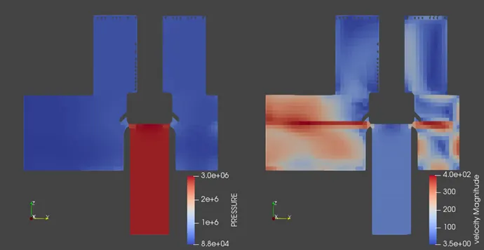
Pressure - Velocity Animation - Case-4- 3mm : https://youtu.be/ZHF_O92-pMk

Pressure – Velocity Contour: Case-5 – 4 mm Lift – With AMR

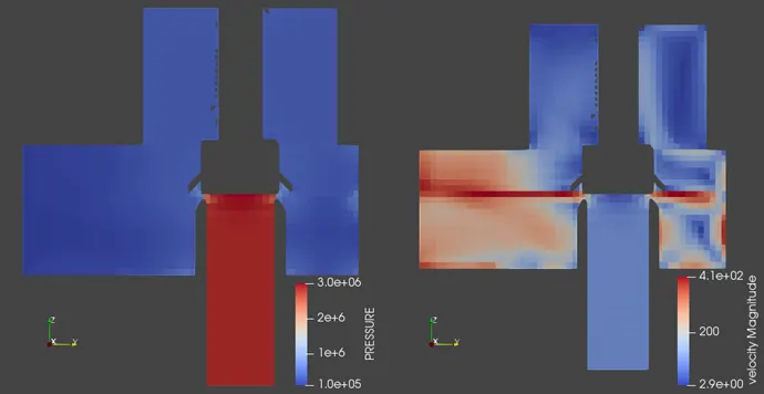
Pressure - Velocity Animation - Case-5- 4mm: https://youtu.be/rln3FAJns70

Pressure – Velocity Contour: Case-6 – 5 mm Lift – With AMR

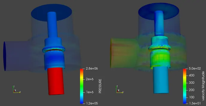
Pressure - Velocity Animation - Case-6- 5mm: https://youtu.be/MF-2Gh3hZyU

Observations for Cases 7: With FSI

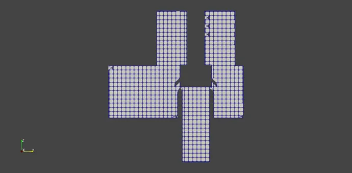
Mesh Formation: Case 7 – With FSI

Force Plot:

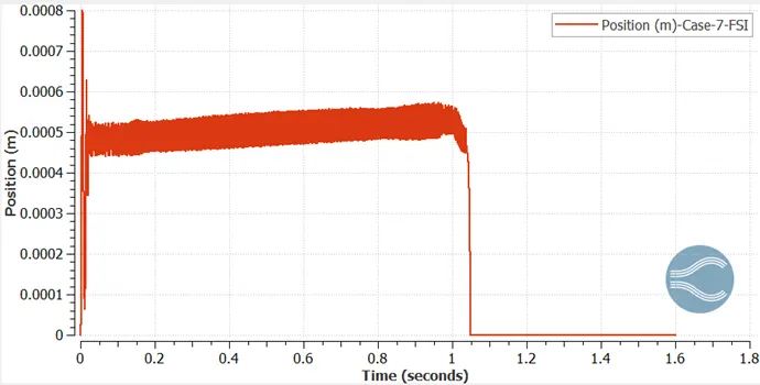
Position Plot:

Pressure-Velocity Case-7- Animation: https://youtu.be/WKnDHqCZ-nU

Results: For Case 1, 2, 3, 4, 5, 6 With / Without AMR -

After running the simulation, the results can be observed as below:

1. Mesh Formations are shown for the Steady State simulation case with AMR and without the use of AMR (Adaptive Mesh Refinement).
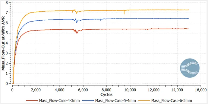
2. The Mass flow rate plots are presented and we can infer that the mass flow has converged. Also the use of AMR effectively captures a fluctuation in the graph near 5000 cycles which cannot be noticed without the use of AMR. The plot clearly shows that with the increase in the lift the mass flow increases because of more space available for the gas.
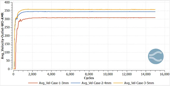
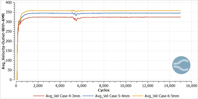
3. From the Velocity plots it is evident that the increase in the lift increases the velocity of the gas passing through the increased space.
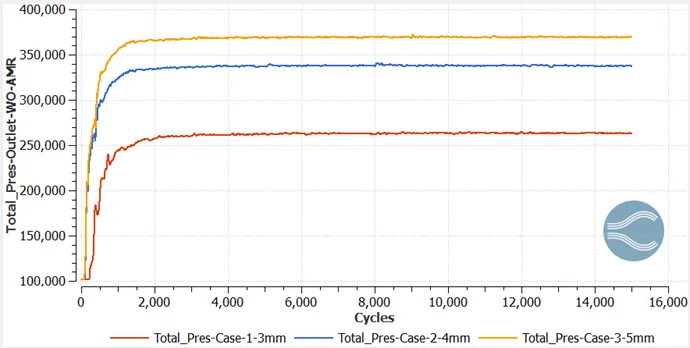
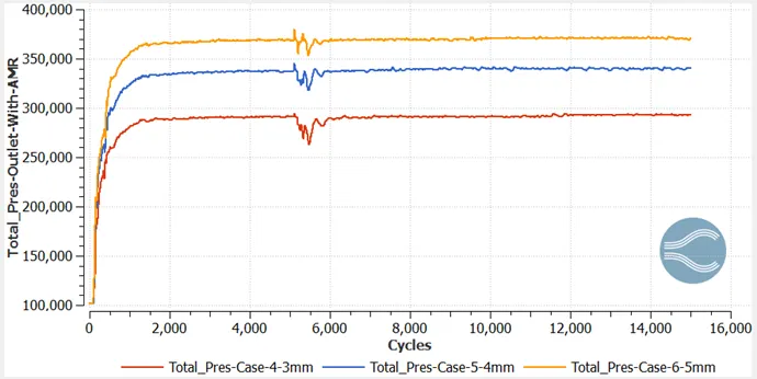
4. From the pressure plot we can observe that the lift increases, velocity increases. Now due to increase in the velocity, total pressure subsequently increases.
5. The Total Cell Counts are shown for the cases run with AMR. The cell count near valve goes as high as 1,25,000.

Results: For Case 7 With FSI -

After running the simulation, the results can be observed as below:

1. Mesh Formations are shown for the Transient Flow simulation.
2. The Force plot is an gives an important observation about the force of 7126 N being applied on the valve. The fluctuating motion can be seen during the initial stages.
3. A variable and reducing pressure profile is used to run the case. The pressure acts against the force applied on the valve due to which up and down motion of the valve can be seen.
4. The position plot shows the varying / fluctuating position of the valve during the face of high pressure application on the valve.

Conclusion:

We can conclude from the simulation using Converge CFD program that:

• Simulation was run for three different valve lifts with and without Adaptive Mesh Refinements on the valve spindle.
• Simulation with FSI method was run and the results obtained can be used to work out the stress on the solid structure.
• The change in the parameters for a flow can be observed from the various animations, plots, contours and profiles.