Week 8- Moving zones approach in Fluent
- Moving zones approach in Fluent.
- What are the approaches by which you would model moving zones?
- Which approach would you use to model unsteady phenomena?
- Aim - To simulate rotary motion for the given geometry.
- Objective - Give detailed explaination of moving zone approaches in fluent.
- Simulate rotary motion for the given geometry in fluent and plot velocity profile of the fluid motion.
- Introduction
- Introduction to moving zone approaches:
- There are two types of motion involved in fluid flow problems.
- Rectilinear motion
- Rotary motion
- Rectilinear motion
- The motion of a body in straight line is known as rectilinear motion.
- It is also known as translational motion.
- A man/car moving on a straight road, a ball dropped from a height, a train traveling on a straight track lays out a straight track.
- Linear motion, also called rectilinear motion, is one-dimensional motion along a straight line .
- Rotary motion
- Rotational motion is defined as the type of motion associated with objects that move in a circular path.
- Types of rotational motion include motion about a fixed axis, motion about an axis in rotation, and a combination of rotational motion and translational motion.
- Two approaches are used to model rotary motion.
- Moving reference frame
- Moving mesh approach
- Moving Reference frame
- Moving reference frame is a steady state method used in CFD to model problems with rotating parts.
- In moving reference case, frame is moving but mesh topology remains same.
- In CFD simulations, MRF is used to simulate fluid flow around rotating components.
- MRF technique makes simulation of the fluid flow in rotating component systems computationally efficient.
- Analyzes flow separation, recirculation, and vortex shedding around rotating machinery.
- The aerospace, automotive and energy industries design and optimize rotary systems using MRF.
- MRF divides the rotation region into stationary reference frames for each rotating component.
- These computational domain reference frames have rotational velocities and axes.
- Each reference frame treats the fluid flow as stationary, which simplifies the simulation.
- The MRF approach means the fluid flow in each reference frame follows the navier stokes equation,coriolis and centrifugal forces.
- Each frame of reference solves the equation separately,while the boundary conditions at the interfaces connect the solutions.
- Types of MRF
- Single moving reference
- Multiple reference frame
- Multiple reference frame uses a mixing plane approach.
- Contact region or the interface.
- This is the region existing in contact between a stationary frame and a moving frame.
- It is the section or region of intersection of two frames.
- In Ansys Fluent, by enabling a moving reference frame in selected cell zones, we can model a problem involving moving parts. when the moving reference frame is activated, the equations of motion are adjusted by incorporating an additional acceleration term due to the transformation of the stationary reference frame to the moving reference frame. By solving these equations in a steady-state manner, the flow around the moving parts can be modeled.
- Data is transferred from one frame to another frame through the interface.
- Methods through which data is transferred through interface are:
- Mass averaging
- Area averaging
- Mixed out approach.
- Moving Mesh approach
- Moving mesh approach is used to model unsteady phenomenon such as vortex induced flows, interaction of vortex with bodies.
- In moving mesh approach, mesh is moving but mesh topology changes with time.
- The moving mesh approach deforms the computational mesh to fit changing geometry.
- The simulation approximately tracks the fluid-solid interface or moving obstacles.
- For every timestep mesh nodes are moved to deal with object shape and vicinity changes.
- The sliding mesh technique simulates fluid structure interaction issues consisting of flow around spinning machinery, oscillating structures and fluid elastic vibrations.
- Setup
- Given geometry
- Import mesh file of the model into setup.
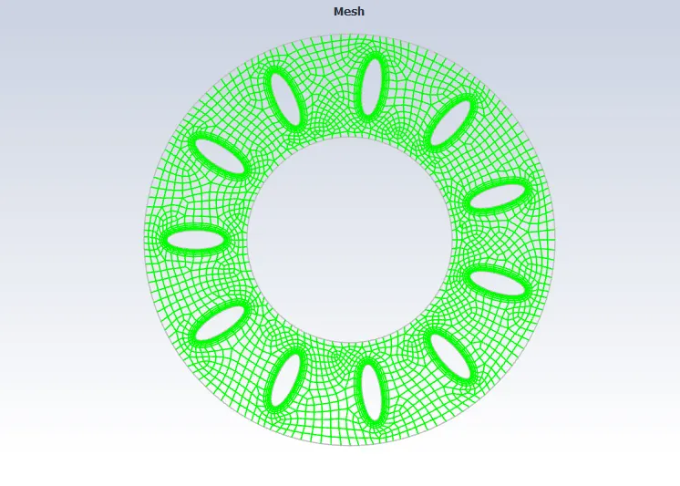
- Preliminary mesh check is done.
- Under the general conditions, Pressure based solver is used. A steady state analysis is performed. Generally with moving refernce frame, steady state studies are conducted.
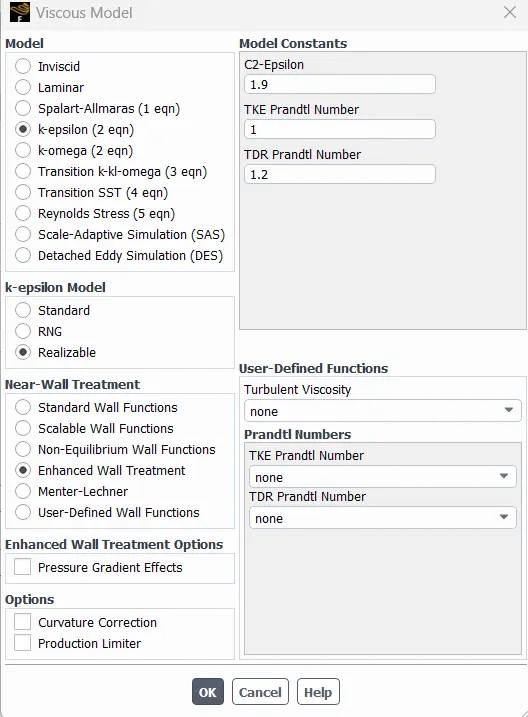
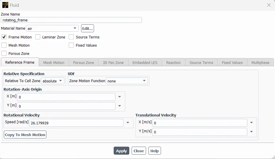
- Cell zone conditions
- Speed = 250 rpm
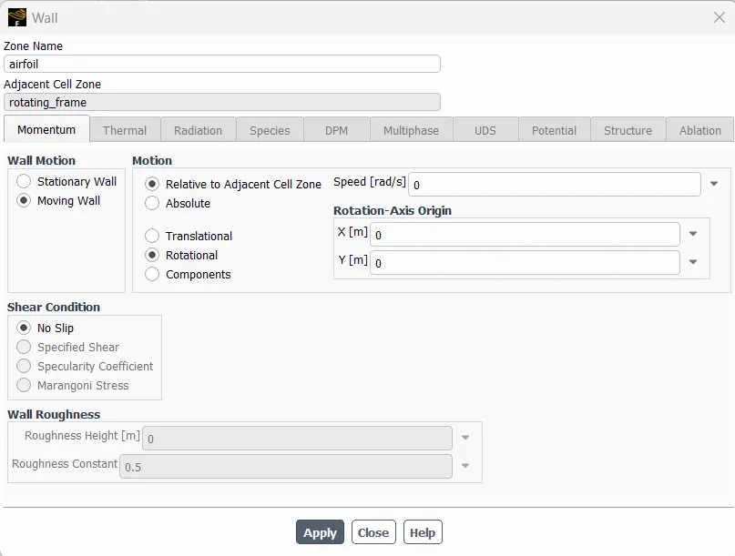
- Boundary Conditions
- For Airfoil
- Solution methods
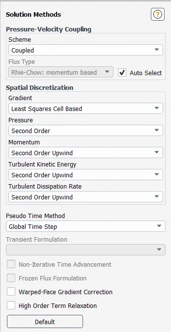
- The solution is set for coupled scheme and second order upwind scheme.
- Hybrid initialization
- Results
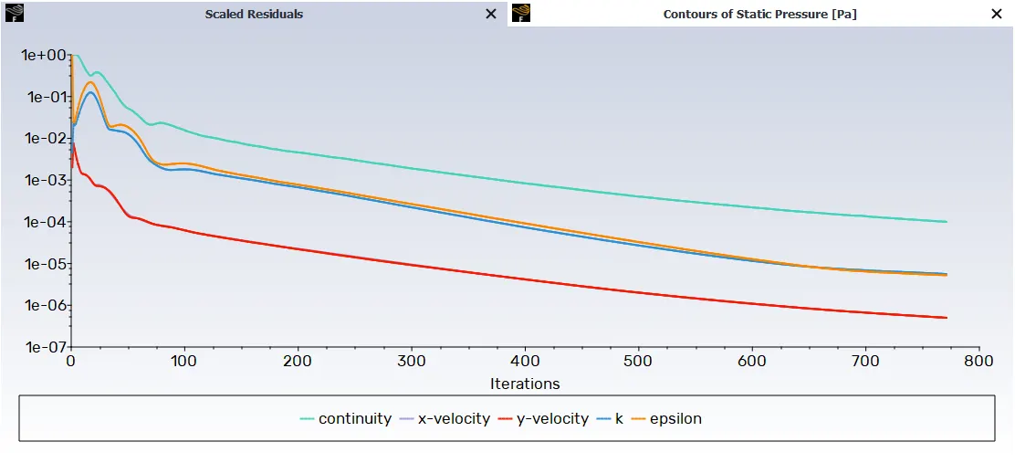
- Residual plot
- Pressure contour
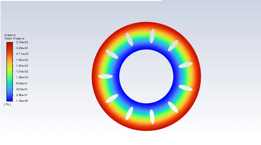
- From the pressure contour we observed that pressure is negative at the inner side of the domain where the suction of air takes place near the centre of the impeller. Maximum pressure is observed at the outer side of the rotating domain and at the leading edge of the airfoils.
- Velocity contour
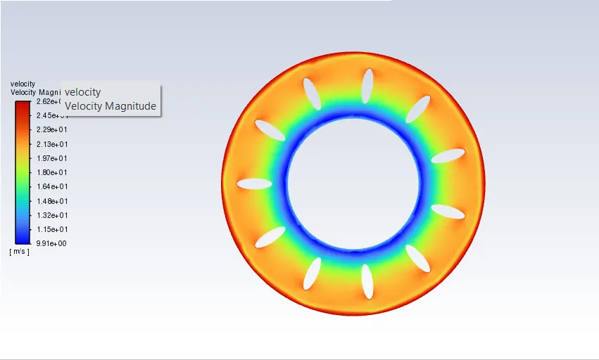
- From the above contour of velocity we can observed that maximum velocity is created at the outer side of the rotating domain and minimun at the rotating inner domain.
- Velocity separation is observed at the leading edge of the airfoils and it decreases from the leading to the trailing edge of the airfoils.
- Velocity vector plot
- Conclusion
- Simulated rotary motion for the given geometry and observed the fluid flow effects by plotting velocity and pressure profile .
- The velocity is maximum (26.2 m/s) at the rotating outer domain and minimum (10m/s) at the rotating inner domain.
- Negative suction pressure is observed in pressure contour near the centre of the impeller.
- Moving mesh approach is very effective method to model unsteady phenomenon.