Week 8- Moving zones approach in Fluent
1. What are the approaches by which you would model moving zones?
The moving cell zone capability in Fluent provides a powerful set of features for solving problems in which the domain or parts of the domain are in motion. It is classified into single rotating frame and multiple rotating or translating reference frames. The single rotating frame option can be used to model flows in turbo-machinery, mixing tanks, and related devices. In each of these cases, the flow is unsteady in an inertial frame because the rotor/impeller blades sweep the domain periodically. However, in the absence of stators or baffles, it is possible to perform calculations in a domain that moves with the rotating part. In this case, the flow is steady relative to the rotating frame, which simplifies the analysis.
If stators or baffles are present in addition to a rotor or impeller, then it is not possible to render the computational problem steady by choosing a calculation domain that rotates with the rotor or impeller. This situation occurs, for example, in turbomachinery applications where rotor and stator blades are in close proximity. Fluent provides three approaches to address this class of problems.
Both the MRF and mixing plane models assume that the flow field is steady, with the rotor-stator or impeller-baffle effects being accounted for by approximate means. These can be acceptable models in cases where the rotor-stator interaction is weak or an approximate solution for the system is desired. The sliding mesh model, on the other hand, assumes that the flow field is unsteady, and hence models the interaction with complete fidelity. This is the model of choice if rotor-stator interaction is strong and a more accurate simulation of the system is desired. However, that because the sliding mesh model requires an unsteady numerical solution, it is computationally more demanding than the MRF and mixing plane models.
in Fluent the typical modelling involves flow in an inertial reference frame. However, Fluent also has the ability to model flows in an accelerating reference frame. In this situation, the acceleration of the co-ordinate system is included in the equations of motion describing the flow. A common example of an accelerating reference frame in engineering applications is flow in rotation equipment. Many such flows can be modelled in a co-ordinate system that is moving with the rotating equipment and thus experiences a constant acceleration in the radial direction. This class of rotating flows can be treated using the rotating reference frame capability in Fluent. Applications include
1. Impellers in mixing tanks
2. Rotating turbomachinery blades
3. Flow in rotating passages,
When such problems are defined in a rotating reference frame, the rotating boundaries become stationary relative to the rotating frame, since they are moving at the same speed as the reference frame.
The various approaches used for modelling moving zones include
1. Moving reference frame model
2. Mixing plane model
3. Sliding mesh model
The Multiple reference frame model:
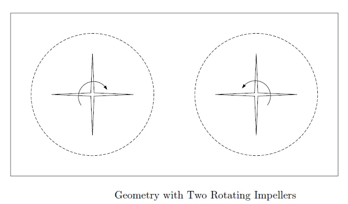
The MRF model is the simplest of the three. It is steady-state approximation in which individual cell zones move at different rotational/translational speeds. This approach is appropriate when the flow at the boundary between these zones is nearly uniform. While the multiple reference frame approach is clearly an approximation, it can provide a reasonable model is the time-averaged flow for many applications. For example, the MRF model can be used for a turbo-machinery application in which rotor-stator interactions are relatively weak, large-scale transient effects are not present and the MRF model can be used. In general, any problems where transients due to rotor-stator interaction are small are candidates for the MRF model. Another potential use of the MRF model, is to compute a flow field that can be used as an initial condition for a transient sliding mesh calculation. this eliminates the need for a startup calculation. The MRF model should not be used, however, if it is necessary to actually simulate the transients that may occur in strong impeller-baffle interactions.
Applications like a mixing tank with a single impeller.
The mixing plane model:
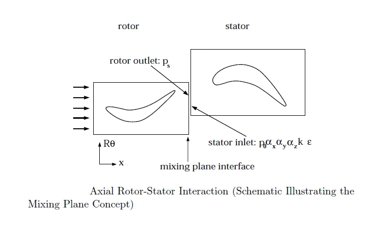
The essential idea behind the mixing plane concept is that each fluid zone is solved as a steady-state problem. At some prescribed iteration interval, the flow data at the mixing plane interface are averaged in the circumferential direction on both the stator outlet and the rotor inlet boundaries. The Fluent implementation uses area-weighted averages. By performing circumferential averages at specified radial or axial stations, ''profiles'' of flow properties can be defined. These profiles - which will be functions of either the axial or radial co-ordinate, depending on the orientation of the mixing plane - are then used to update boundary conditions along the two zones of the mixing plane interface. Applications include radial rotor-stator interaction setup.
Sliding mesh model:
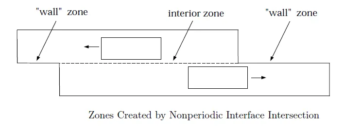
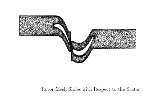
when a time -accurate solution for rotor-stator interaction is desired, sliding mesh model is used to compute the unsteady flow field. it is the most accurate method for simulating flows in multiple moving reference frames, but also the most computationally demanding. Most often, the unsteady solution that is sought in a sliding mesh simulation is time-periodic. That is the unsteady solution repeats with a period related to the speeds of the moving domains. However, you can model other types of transients, including translating sliding mesh zones. The flow situations where there is no interaction between stationary and moving parts, the computational domain can be made stationary by using a rotating reference frame. When transient rotor-stator interaction is desired, sliding mesh is used. here, two or more cell zones are used. Each cell zone is bounded by at least one ''interface zone'' where it meets the opposing cell zone. The interface zones of adjacent cell zones are associated with one another to form a grid interface. The two cell zones will move relative to each other along the grid interface.
2. Which approach would you use to model unsteady phenomena?
The moving mesh/ sliding mesh approach is used to model the unsteady phenomenon. Time-periodic solution can be arrived by using the sliding mesh/moving mesh technique.
3. Simulation of rotary motion:
Viscous model: K-Omega SST model is selected for the moving zones approach.
Cell zone: Rotating frame is set at 250 rpm with frame motion.
Fluid: Air with constant density.
Boundary conditions: The inner and outer lines are kept as walls and The rotating frame is kept as interior.
Mesh:
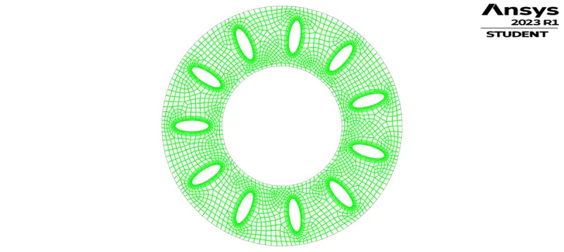
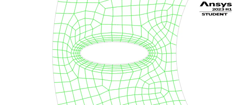
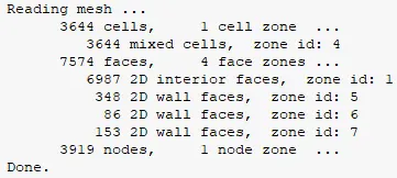
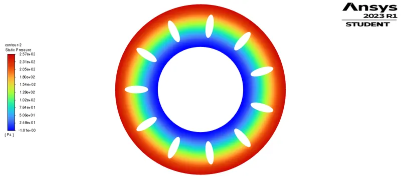
Pressure profile:
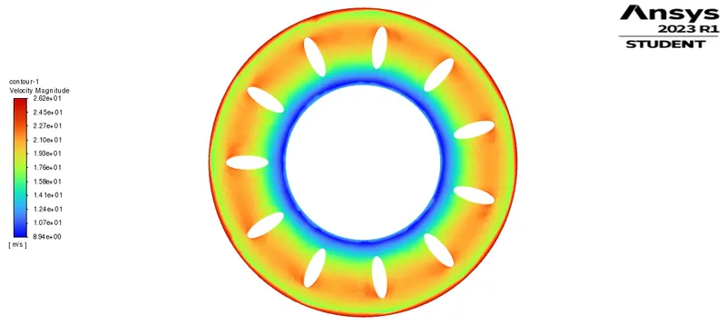
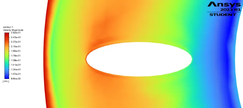
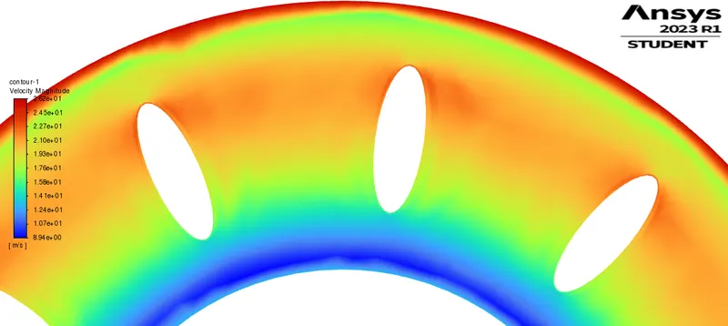
Velocity profile:
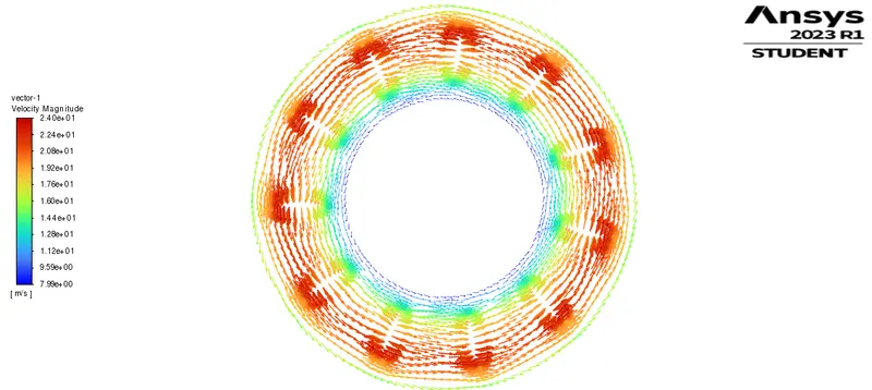
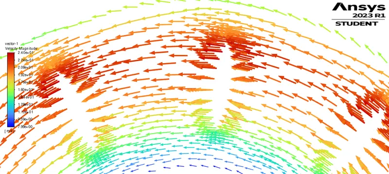
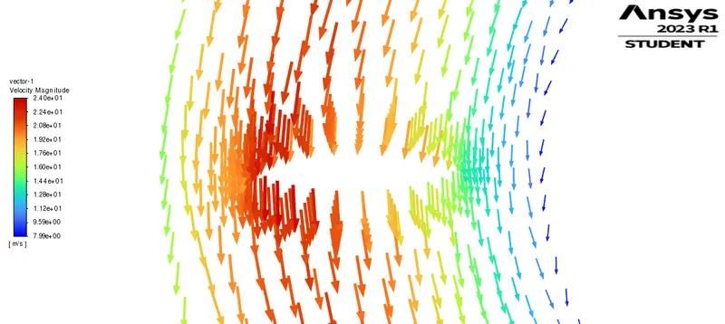
Vector plot:
Inference:
Since there is one rotating cell zone in the domain, moving reference frame approach is used. The frame is set to rotate at 250rpm. The airfoil cell zones are made stationary with the frame in motion. From the contours, it can be observed that the fluid around the outer wall has more pressure than the inner wall. The inner wall has low pressure which steadily increases while moving outwards on the frame. The velocity contours shows that there is higher velocity on the outer wall than the inner wall. It is also seen there is an increased velocity on the outer end of the airfoil from the vector plot. There is a steady increase in velocity while moving outwards towards the rotating frame. The vector plot also shows that the fluid flow on the outermost zone has low velocity than the fluid flow near the airfoil.