Week - 8 Mass Scaling

AIM:

To perform the simulation by reducing and stabilizing the run time with the help of mass-scale factor.

BASIC THEORY:

MASS SCALING: In an explicit method, the time step usually is very small to maintain numerical stability. However, small step prevents this method from being useful for routine analysis work.

To reduce CPU cost and improve the performance , mass scaling is often used to increase the time step size in each cycle . Several methods can be used with LS-DYNA to accomplish this. The simplest method is to use a large mass density for the blank.

Alternatively, the user may specify the desired minimum time step size in *CONTROL_TIMESTEP.

Mass-scaling refers to a technique whereby non-physical mass is added to a structure in order to achieve a larger explicit time step. One can employ mass scaling manually by artificially increasing the material density of the parts you want to mass-scale. This manual form of mass scaling is done independently of the automatic mass-scaling invoked with DT2MS in *CONTROL_TIMESTEP. When DT2MS is input as a negative value, mass is added (with a safety factor: see note at end of this file) only to those element whose time step would otherwise be less than TSSFAC .

By adding mass to these elements, their time step becomes equal to TSSFAC. The trend is that the smaller the TSSFAC, the greater the added mass. In return, stability may improve as TSSFAC is reduced.

If stability is a problem with the default TSSFAC of 0.9, try 0.8 or 0.7. If you reduce TSSFAC , you can increase DT2MS proportionally so, that their product and hence time step is unchanged.

The difference between using a positive or negative number for DT2MS in *CONTROL_TIMESTEP is follows:

Negative: Mass is added to only those element whose time step would otherwise be less than TSSFAC . When mass scaling is appropriate.

Positive: Mass is added or taken away from element , so that the time step of every element is the same. My opinion is there is no advantage to using this method over the negative DT2MS method.

PROCEDURE:

CASE 1: EXPLICIT ANALYSIS(WITH MASS SCALE)

STEP 1: IMPORT .k FILE

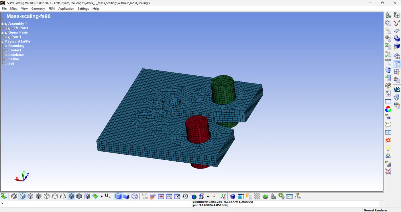
STEP 2: RUN THE DEFAULT FILE.

STEP 3: RUN ALL CHANGED TIME-STEP FILE ONE BY ONE.

DT2MS and TSSFAC are the parameters , that transform the time step and run time of the simulation. In order to that , we could change these values in each iteration to obtain an optimized run time with a stable solution and to make sure mass scaling accomplishes 8%.

1. Iteration 1, DT2MS=-3.5e-5, TSSFAC= 0.9, DTINIT=0.001

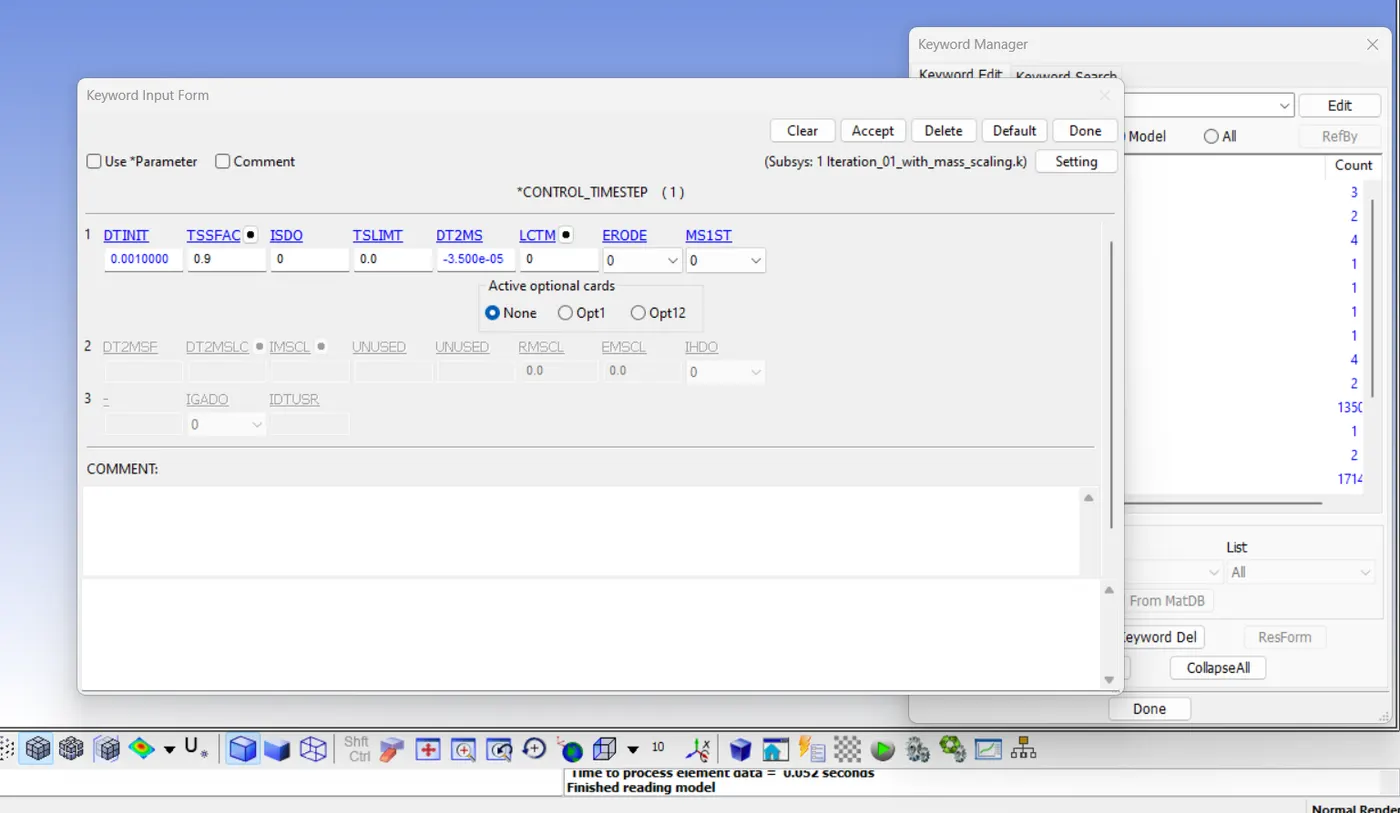
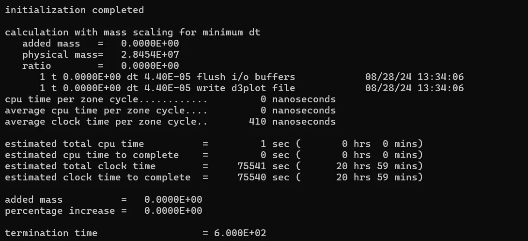
From the above image computational time is 20hrs 59 min .As a result , there is no mass added with given DT2MS. This can be varied by changing values of DT2MS and TSSFAC.

2. Iteration 2, DT2MS=-3.5e-5, TSSFAC=0.7, DTINIT=0.001

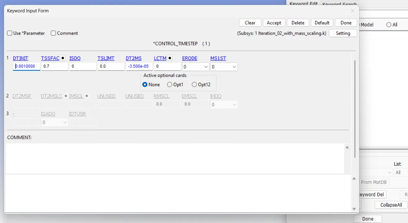
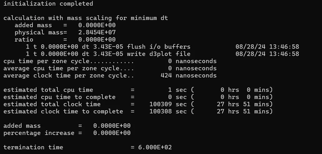
From the above image computational time increased by 20hrs 59min to 27hrs 51mins , as a change in TSSFAC=0.7 leads to a rise in timing. However , we can see that the mass scale factor still pretains to zero factor.

3. Iteration 3, DT2MS=-6.5e-5, TSSFAC=0.7, DTINIT=0.001

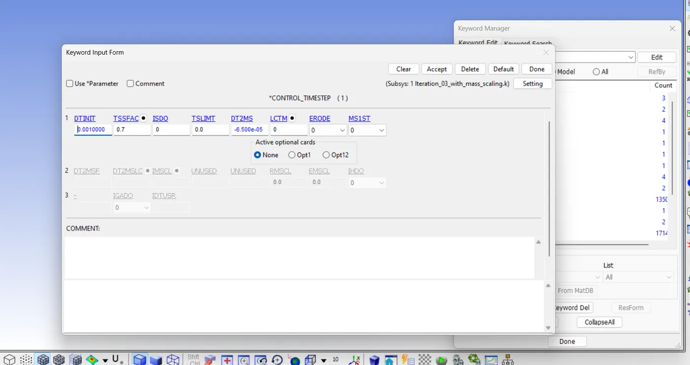
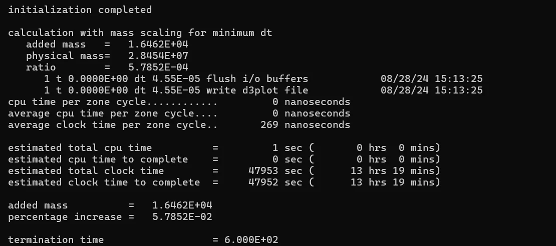
From the above image computational time decreased rapidly from 27hrs 51mins to 13hrs 19mins .There is a considerable decrease in computational time .

The mass added with this DT2MS and TSSFAC value percentage of mass increase in 5.7852e-02.

4. Iteration 4, DT2MS=-6.5e-4, TSSFAC=0.7, DTINIT=0.001

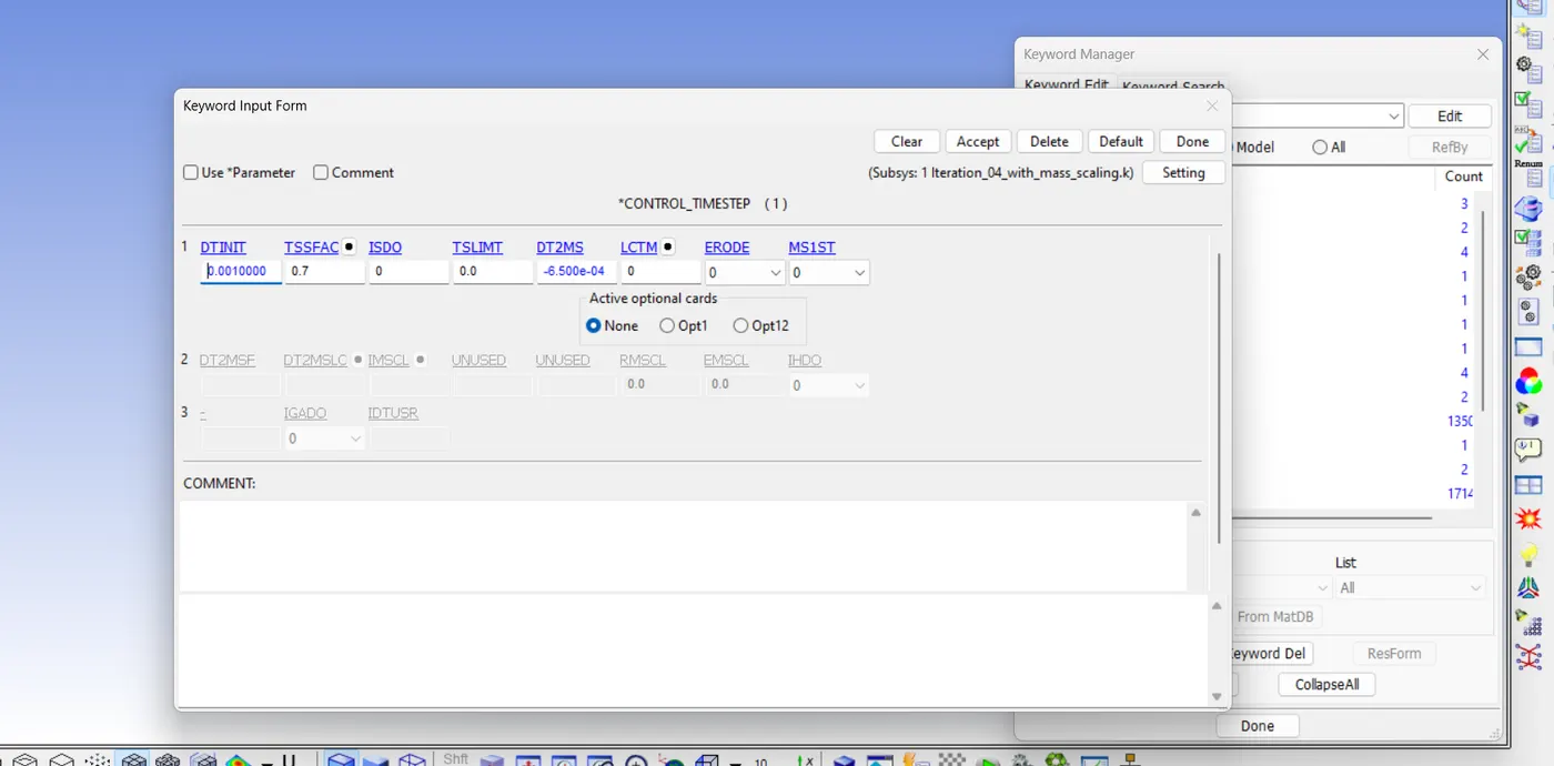
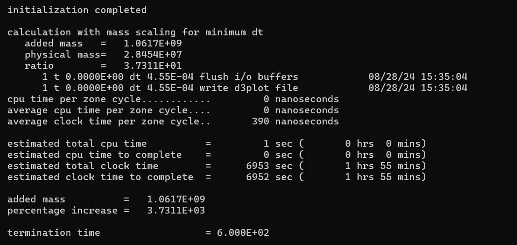
Computational time decreased rapidly from 13hrs 19mins to 1hrs 55mins . There is a considerable decrease in computational time.

The mass added with values of DT2MS and TSSFAC with a percentage of mass increase in 3.7311E+03.

Since the added mass exceeding the limit , the energy values also vary considerably, values need to be reduced.

5. Iteration 5, DT2MS=-1.5e-4, TSSFAC=0.7, DTINIT=0.001

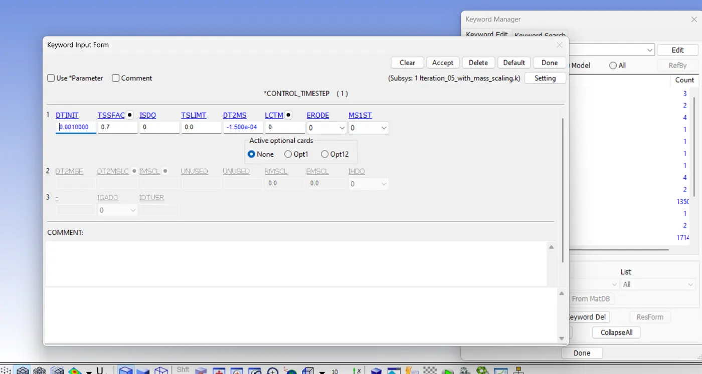
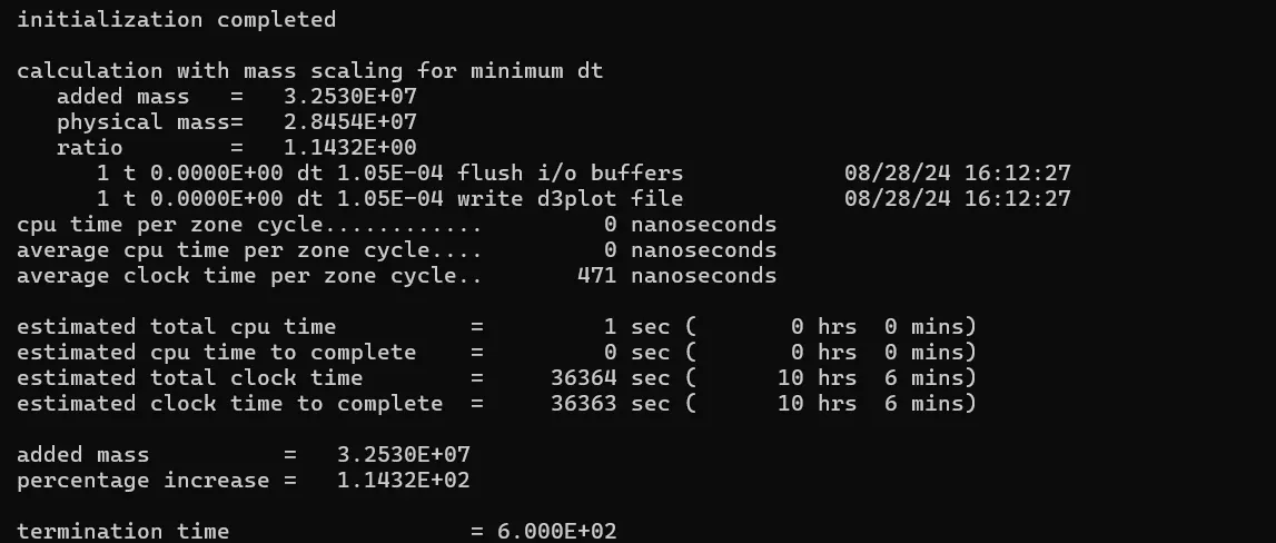
Computational time increased rapidly from 1hrs 55mins to 10hrs 6mins .

The mass added with a default values of TSSFAC and DT2MS with a percentage of mass increase in 1.1432E+02.

Since the added mass exceeding the limit , the energy values also vary considerably. values need to be reduced.

6. Iteration 6, DT2MS=-1.1e-4, TSSFAC=0.7, DTINIT=0.001

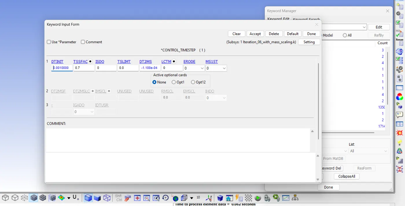
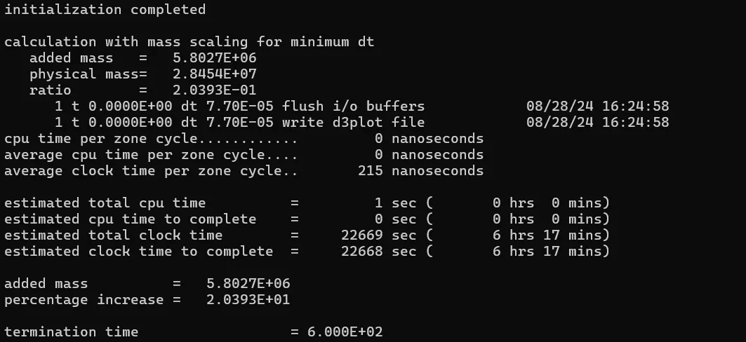
Computational time decreased slightly from 10hrs 6mins to 6hrs 17mins .

The mass added with a default values of TSSFAC and DT2MS with a percentage of mass increase in 2.0393E+01.

7.Iteration 7, DT2MS=-1.01e-4, TSSFAC=0.7, DTINIT=0.001

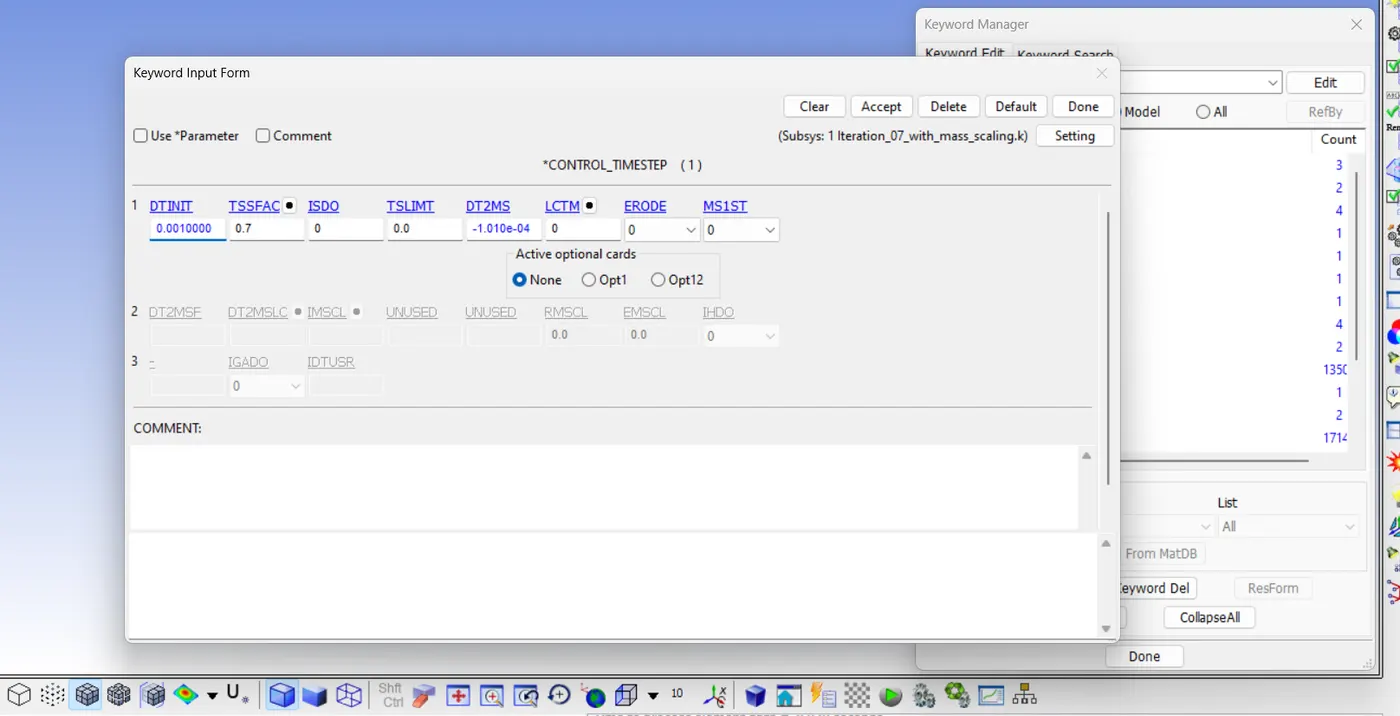
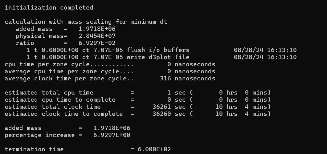
Computational time increased from 6hrs 17mins to 10hrs 4mins .

The mass added with a default values of TSSFAC and DT2MS with a percentage of mass increase in 6.9297E+00.

Since the added mass has reached nearly the required limit, the energy values vary considerably , the values need to be reduced slightly.

8. Iteration 8, DT2MS=-1.02e-4, TSSFAC=0.7, DTINIT=0.001

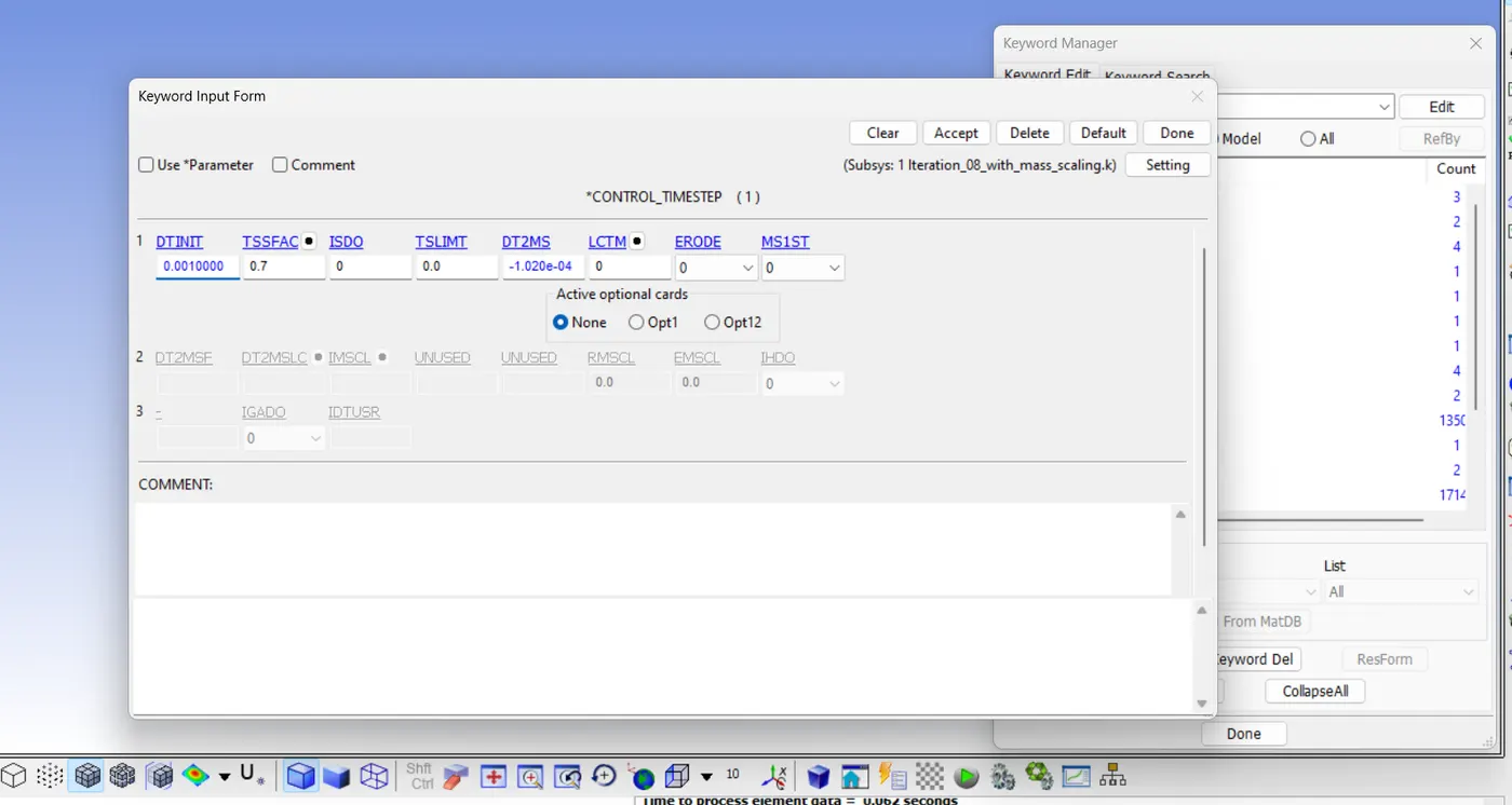
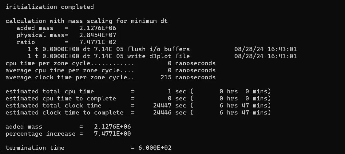
Computational time decreased from 10hrs 4mins to 6hrs 47mins .

The mass added with a default values of TSSFAC and DT2MS with a percentage of mass increase in 7.4771E+00.

Since the added mass has reached the required limit.

CASE 2: IMPLICIT ANALYSIS.

STEP 1:Define *CONTROL_IMPLICIT_AUTO card.

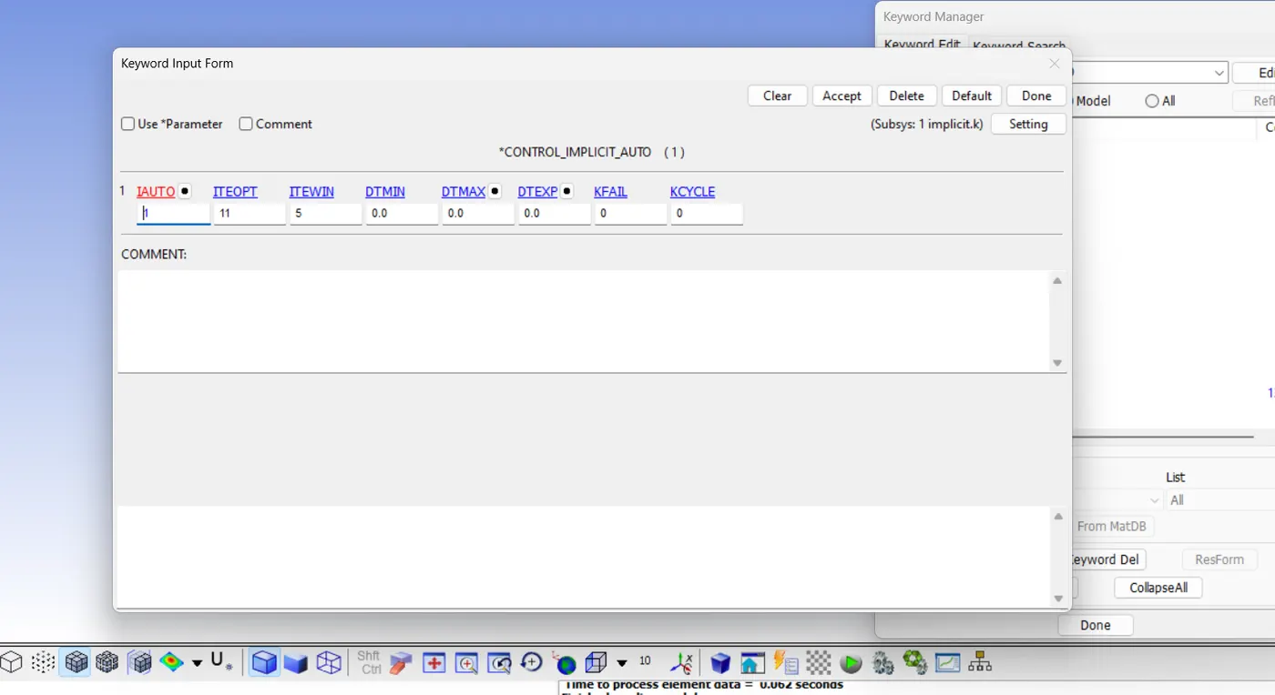
IAUTO=1, ITEOPT=11, ITEWIN=5

STEP 2:Define *CONTROL_IMPLICIT_GENERAL.

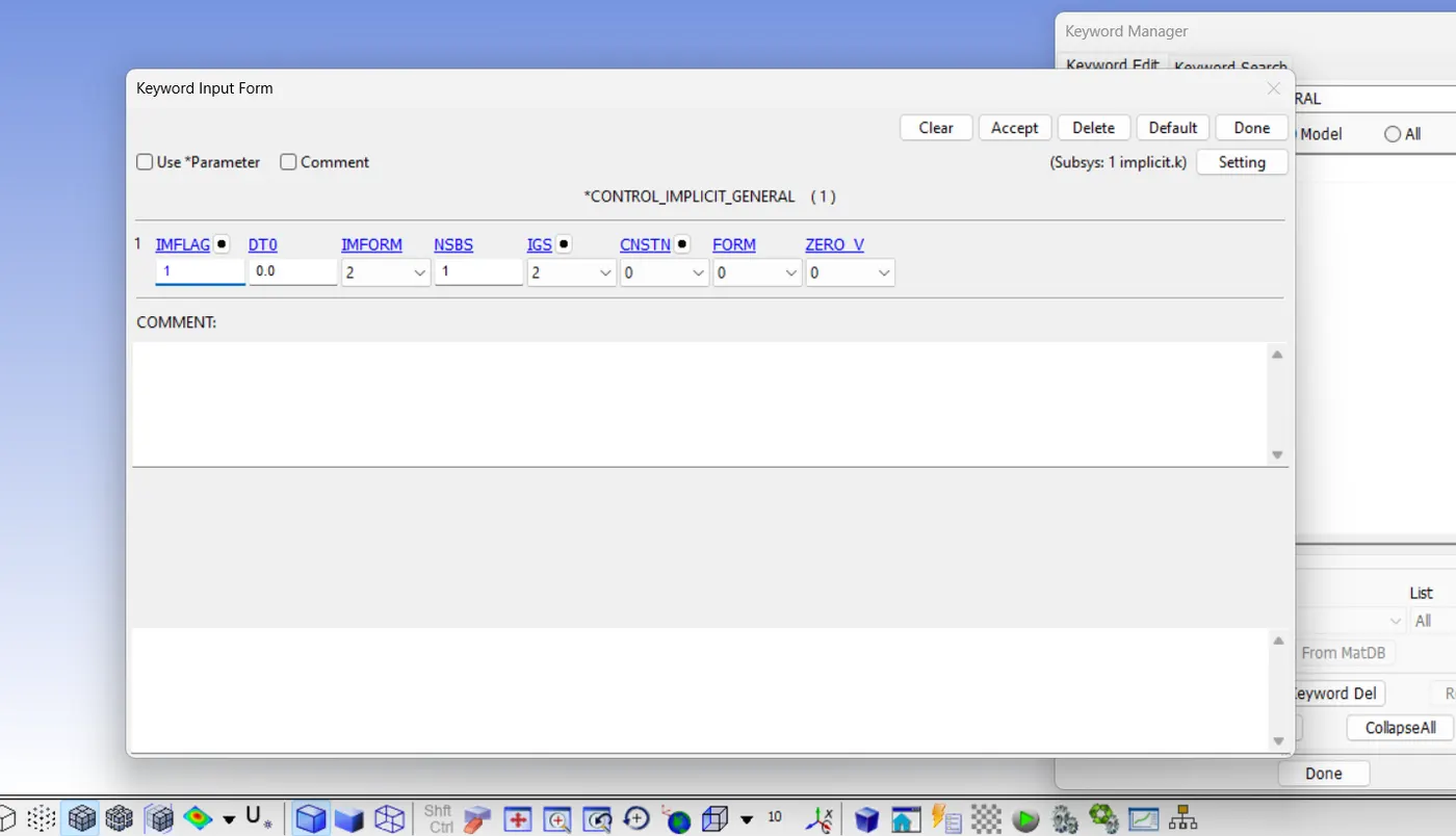
IMFLAG=1, DTO=0, IMFORM=2, NSBS=1, IGS=2

THEN RUN THE FILE...........

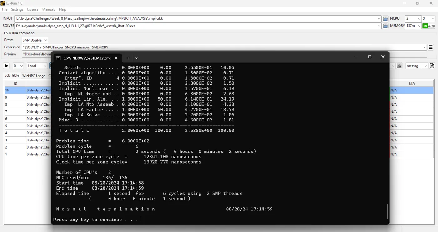
There is no mass added during the computational time, also attached with *CONTROL_TIMESTEP.

In this method, the computational time is less than 1 second maximum for this set up case.

CONCLUSION.........

1. The objective of mass scaling is achieved for the given model by varying the values of DT2MS and TSSFAC using trial and error method.

2.The values of DT2MS and TSSFAC does not affect the run time required to complete the simulation for implicit analysis.

3.The concept of mass scaling and its necessity is in explicit analysis only.