Week - 8 Mass Scaling

Skill-lync assignment 8

Aim: The objective of this assignment is to operate on the given component and minimise its run time via mass scaling, without compromising on stability. The model is to be worked on in three iterations. The first iteration is to be simulated in its original state. The second iteration is to be formulated with optimal mass scaling. The third iteration is to be solved with the implicit solver.

Case setup: The given component is a steel plate with solid pins running through 2 holes that are pulled apart to generate bending stress. The component is illustrated below.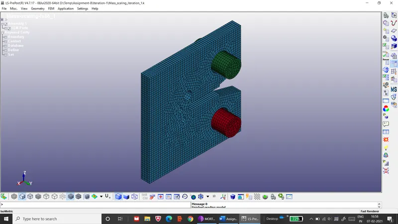

Figure 1: Plate and pins assembly

The lower pin is fixed, while the upper pin moves upwards.

Procedure: The component is worked on through the following series of steps: -

1. The component is first run with LS-Run.
2. The output file is checked for the error that caused error in termination observed.
3. The memory allocated in the keyword ID is deleted and the file is run again. This time, the total run time is estimated to be 149874 sec (1 day, 17 hrs, 37 min and 54 sec).
4. In the CONTROL>TERMINATION keyword, the ENDMAS parameter is set as 8, so that the simulation is terminated when added mass exceeds 8%.
5. In the CONTROL>TIMESTEP keyword, the MS1ST parameter is set as 1 so that mass scaling is applied only during the first time step. Also, the IMSCL (flag for selective mass scaling) parameter is set as 1 so that mass scaling is not applied to rigid components.
6. In the same keyword, the DT2MS (time step size for mass scaled solutions) parameter is set to various values and the resultant computaton times are noted and compiled.
7. The keyword has a copy made that is used as the third and final iteration.
8. The CONTROL>TIMESTEP keyword is deleted and replaced by the CONTROL>IMPLICIT_GENERAL keyword. In this keyword, the initial time step is varied and the overall computaton times are noted.
9. The CONTROL>IMPLICIT_AUTO keyword is added to control the time step variation. An optimal number of iterations are set in the ITEWIN parameter as 11, and the minimum allowable time (DTMIN) is varied to observe the effect on computation time.

Results: The first iteration, i.e. the original component had an estimated computation time of 149874 sec (1 day, 17 hrs, 37 min and 54 sec). Compared to this, the second iteration has a very complex corelation between the computation time step, the mass scaling and the minimum time step, as plotted below.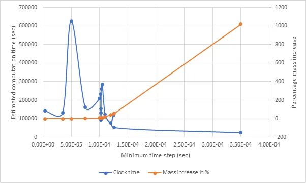

Figure 2: Computation time vs. minimum time step plot for explicit analysis

It shows a well defined increase in mass scaling at roughly the 0.1 ms time step mark. This shows that the use of mass scaling for reducing computation is clearly limited to small time step increments. This is easier to see since the MS1ST settings for the second iteration causes mass scaling only during the first time step. The actual computation time is highly inconsistent. The time step varies during the simulation since the MS1ST setting only works during the first time step and can decrease during the simulation. Generally though, the computation time reduces with increase in time step. Ultimately, the optimal time step for minimum time step with mass scaling being limited to 8% is seen to be 0.1028 ms. The computational time for this time step is estimated to be 91973 sec (1 day, 1 hr, 32 min, and 53 sec), almost 39% lower than the original model. The range of time step for which computational time is lower, however, is very narrow.

The third iteration made use of implicit analysis, which was a better fit for the component, given the low velocity boundary condition that makes this a quasi-static scenario. The overall computation times were dramatically lower than those of the second iteration. The following plot shows the relation between computation time and initial time step.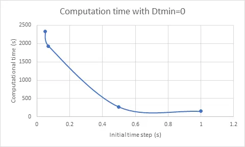

Figure 3: Computation time vs. initial time step plot for implicit analysis

It shows that computation time is inversely proportional to time step. Overall, the greatest computation time was 40 min, while the lowest was 2 min 31 sec. Based on this plot, it is apparent that the optimal value of initial time step is roughly 0.65 sec. Raising the minimum time step also reduces the computation time due to the inverse proportionality between the two. It is observed that for initial time step of 0.05 sec, change in minimum time step does not influence computation time. This points to time step in the simulation reaching a stable value of 0.05 sec or close. While this might seem to be the result of time step control by the IMPLICIT_AUTO keyword for maintaining optimal number of iterations per step (11), the actual number of iterations is observed to be 2. It is more likely that this value of time step is minimum value attained due to mesh deformation during the simulation.

The observed stress in all the cases for the third iterations were mostly consistent, with a maximum value of about 3.8 X 10^-7 Pa. Larger time steps caused the stress plot to show more variation from linear behavior, as shown in the plot below for time step of 1 sec.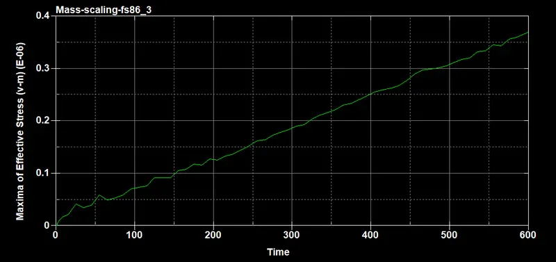

Figure 4: Stress history plot for initial time step of 1 sec

This shows the need for small time steps for generating accurate results. Possibly due to the low value of mposed velocity. This stress has a very low value and is develops almost uniformly within the plate.

Conclusion: The mass scaling and time step scaling has been successfully demonstrated in the given component. These methods have shown their use in computation time reduction. The suitability of explicit and implicit analyses were also demonstrated for the given component, which showed greater affinity for implicit analysis.