Week - 8 Mass Scaling

OBJECTIVE :

To use the mass scaling to reduce the runtime of a model and ensure the stability of mass scaling. The hard limit on mass scaling is 8% and stability should be completely intact. This means that two simulations, one with mass scaling and one without should behave exactly the same way. The submission should contain the trials for mass scaling and the data generated henceforth. Both the DT and TSSFAC parameters should be optimized.

We supposed to take the attached model and do trial and error for mass scaling. Once the mass scaling objective is reached, a histogram should be plotted to compare the runtime with mass scaling trials. Finally, we need to run the same model using implicit solver with necessary changes and compare implicit and explicit runtime.

Theory:

Mass-scaling refers to a technique whereby nonphysical mass is added to a structure in order to achieve a larger explicit timestep. Anytime you add nonphysical mass to increase the timestep in a dynamic analysis, you affect the results (think of F=m*a). Sometimes the effect is insignificant and, in those cases, adding nonphysical mass is justifiable. Examples of such cases may include the addition of mass to just a few small elements in a noncritical area or quasi-static simulations where the velocity is low and the kinetic energy is very small relative to the peak internal energy. In the end, it's up to the judgement of the analyst to gage the affect of mass scaling. You may have to reduce or eliminate mass scaling in a second run to gage the sensitivity of the results to the amount of mass added.

One can employ mass scaling in a selective manner by artificially increasing material density of the parts you want to mass-scale. This manual form of mass scaling is done independently of the automatic mass scaling invoked with DT2MS in *CONTROL_TIMESTEP.

When DT2MS is input as a negative value, mass is added only to those elements whose timestep would otherwise be less than|DT2MS|. By adding mass to these elements, their timestep becomes equal to |DT2MS|. An infinite number of combinations of TSSFAC and DT2MS will give the same product, i.e., timestep but the added mass will be different for each of those combinations. The trend is that the bigger |DT2MS| (and the smaller TSSFAC while TSSFAC*|DT2MS|=const), the greater the added mass. In return, stability may improve as TSSFAC is reduced (just as in non-mass-scaled solutions). If stability is a problem with the default TSSFAC of 0.9, try 0.8 or 0.7. If you reduce TSSFAC, you can increase |DT2MS| proportionally so that their product, and hence timestep, is unchanged.

The difference between using a positive or negative number for DT2MS in*CONTROL_TIMESTEP is as follows:

Negative: Mass is added to only those elements whose timestep would otherwise be less than TSSF*abs(DT2MS). When mass scaling is appropriate, I recommend this method.

Positive: Mass is added or taken away from elements so that the timestep of every element is the same. My opinion is there is no advantage to using this method over the negative DT2MS method and I find it harder to rationalize.

The parameter MS1ST in *CONTROL_TIMESTEP controls whether mass is added only once during initialization (MS1ST=1) or anytime as necessary to maintain the desired timestep specified via DT2MS (MS1ST=0).

You can use ENDMAS in *CONTROL_TERMINATION to stop the calculation after a certain amount of mass has been added (active for automatic mass scaling only).

PROCEDURE :

• First we need to run the given .k file model without changing DT2MS AND TSSFAC Values and the estimated total run time obtained is 26 hours and 49 mins.
• Now keeping the TSSFAC value to 0.9 with changing D2TMS value with small interval steps the result obtained are shown below.

For TTSFAC = 0.9 and D2TMS = -3.5E-5

estimated total time obtained is 26 hours 49 mins.

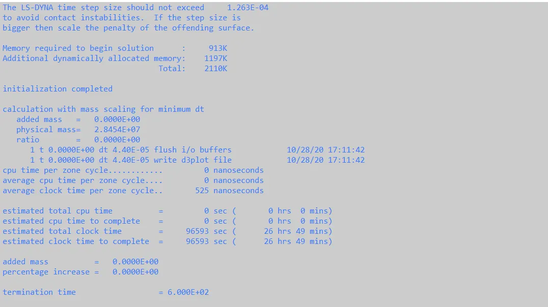
For TSSFAC = 0.9 and D2TMS = -3.0e-5

estimated total time obtained is 22 hours 21 mins

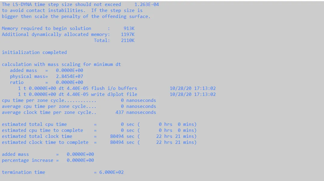
For TSSFAC = 0.9 and D2TMS = -2.5E-5

estimated total time obtained is 24 hours 25 mins

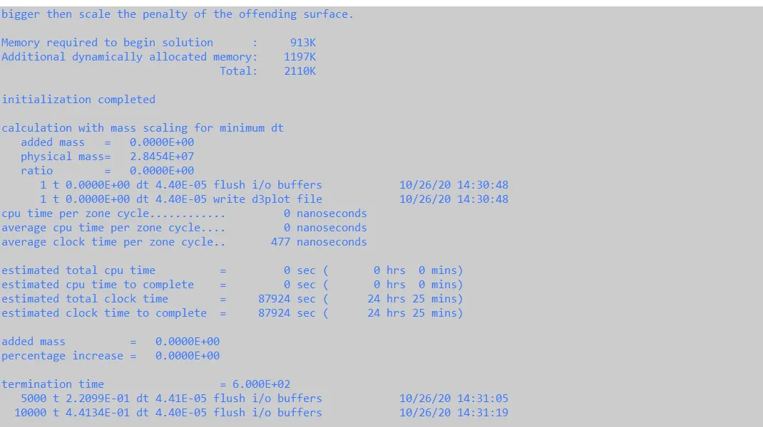
For TSSFAC = 0.9 and D2TMS = -2E-5

estimated total time obtained is 24 hours 25 mins

For TSSFAC = 0.9 and D2TMS = -1.5e-5

estimated total time obtained is 26 hours 29 mins

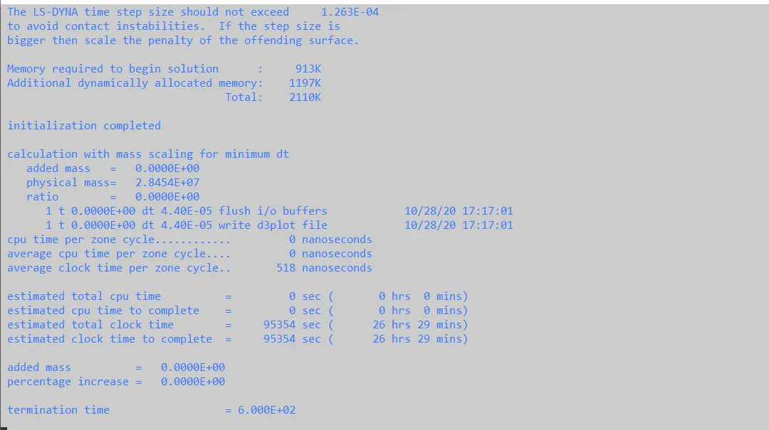
For TSSFAC = 0.9 and D2TMS = -1e-5

estimated total time obtained is 28 hours 12 mins

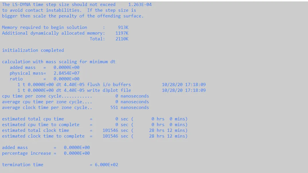
For TSSFAC = 0.9 and D2TMS = -0.5E-5

estimated total time obtained is 24 hours 25 mins

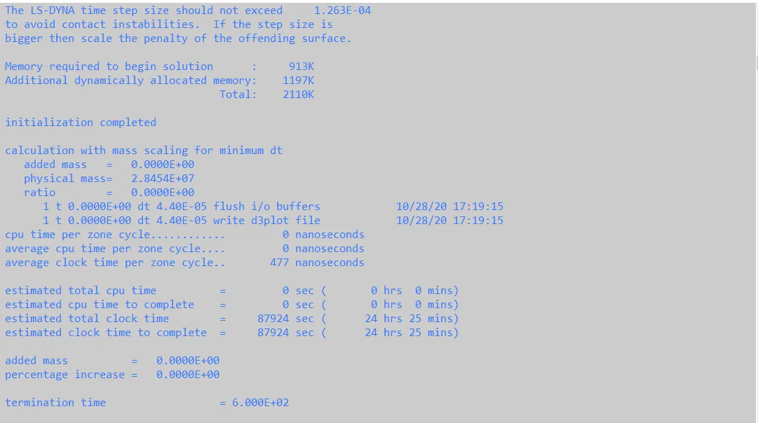
For TSSFAC = 0.9 and D2TMS = -5E-5

estimated total time obtained is 23 hours 2 mins

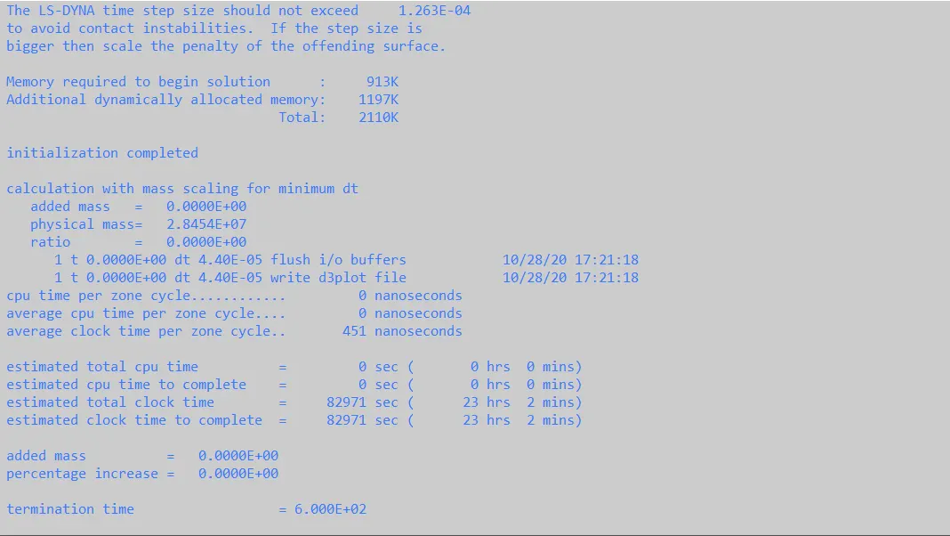
For TSSFAC = 0.9 and D2TMS = -6E-5

estimated total time obtained is 19 hours 21 mins and percentage increase of mass is 0.0227

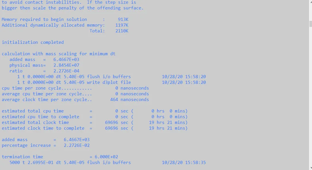
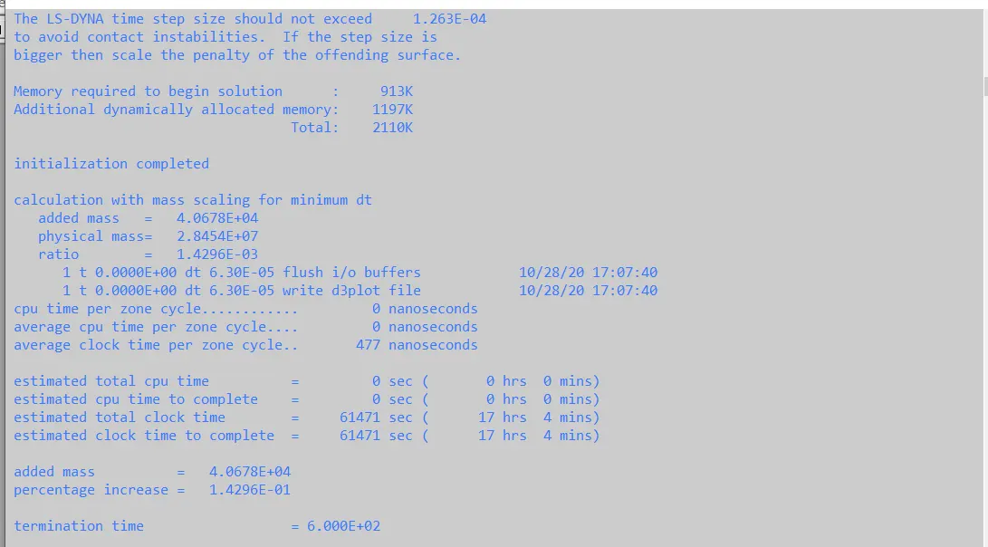
For TSSFAC = 0.9 and D2TMS = -7E-5

estimated total time obtained is 17 hours 4 mins and percentage increase of mass is 0.142

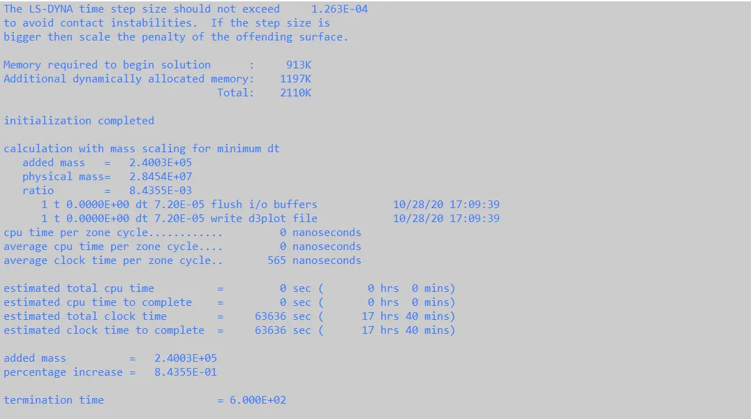
For TSSFAC = 0.9 and D2TMS = -8E-5

estimated total time obtained is 17 hours 40 mins and percentage increase of mass is 0.843

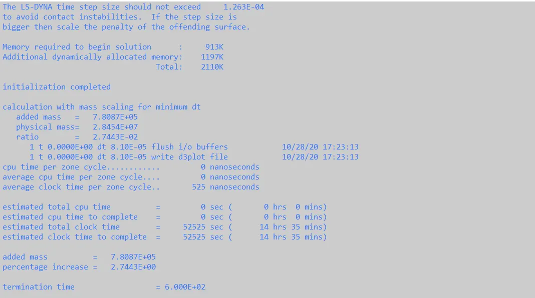
For TSSFAC = 0.9 and D2TMS = -9E-5

estimated total time obtained is 14 hours 35 mins and percentage increase of mass is 2.744

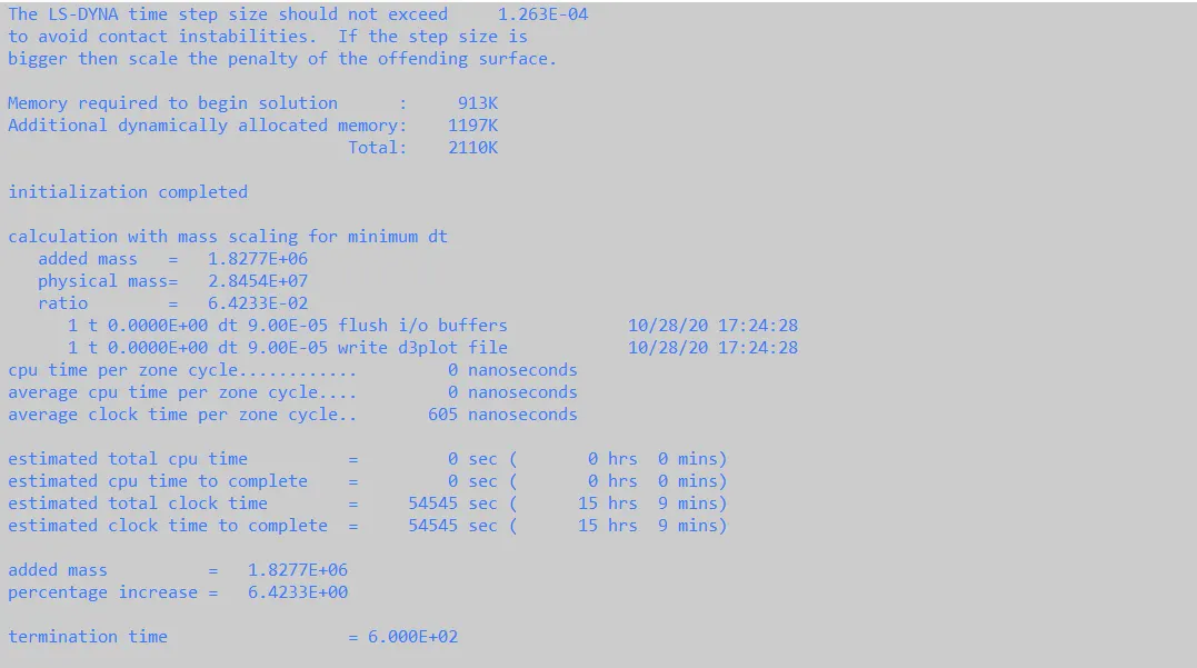
For TSSFAC = 0.9 and D2TMS =-10E-5

estimated total time obtained is 15 hours 9 mins and percentage increase of mass is 6.423

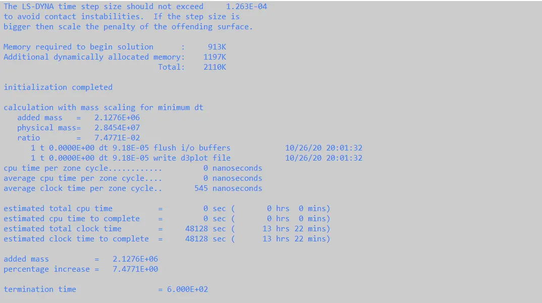
For TSSFAC = 0.9 and D2TMS = -10.2E-5

estimated total time obtained is 13 hours 22 mins and percentage increase of mass is 7.477

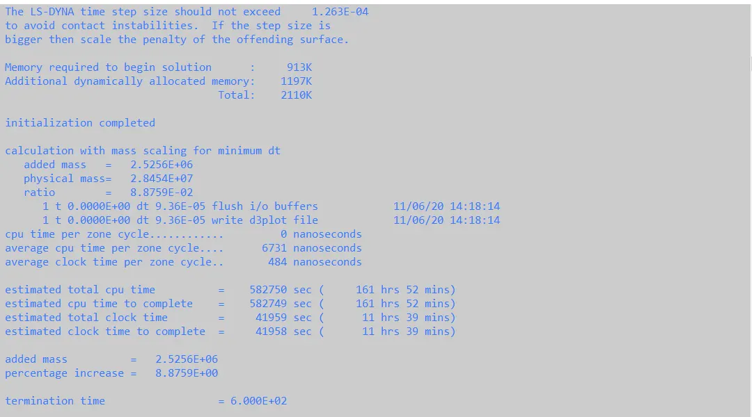
For TSSFAC = 0.9 and D2TMS = -10.4E-5

estimated total time obtained is 11 hours 39 mins and percentage increase of mass is 8.875. As 8% is the limit of percentage of mass adding in the given problem so mass adding as been stopped here.

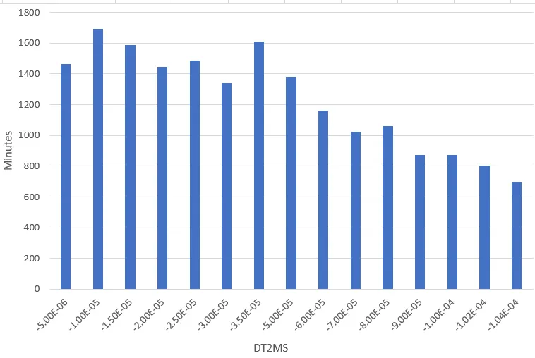
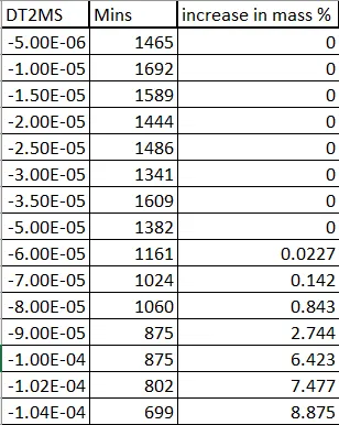
From the above plots we can see the vary of time w.r.t DT2MS value. the estimated total time obtained in the simulation is a rough estimation. The actual values will be lesser then the values shown here. Estimated total time differs from system to system this is because it is dependent on the configuration of the system and the running application at the time of the simulation. the limiit of mass adding percentage is 8% so the problem is stopped at -10.4e-5 where mass percentage increase is 8.875

Now we will check the different values for TSSFAC

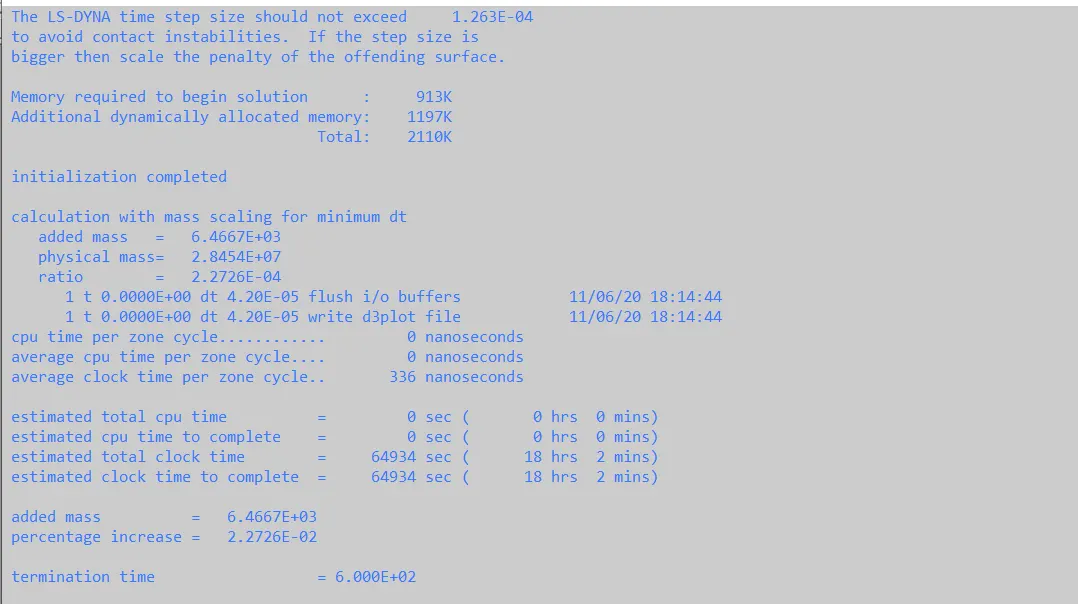
For TSSFAC = 0.8 and D2TMS = -6E-5

For TSSFAC = 0.7 and D2TMS = -6E-5

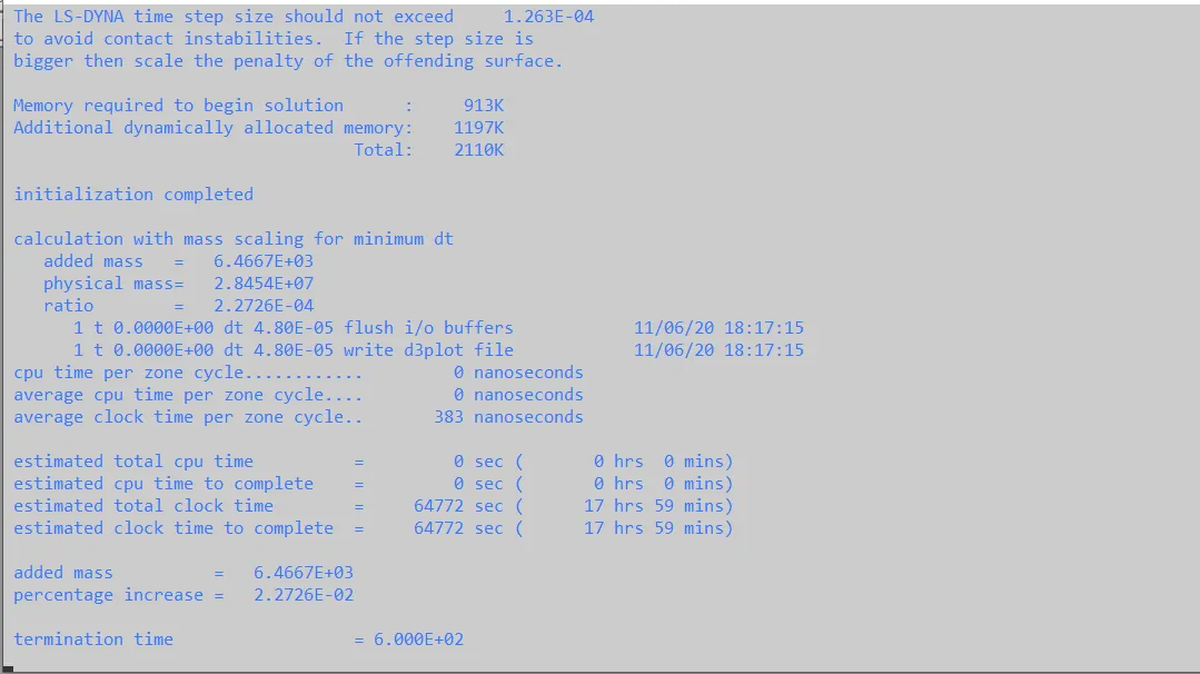
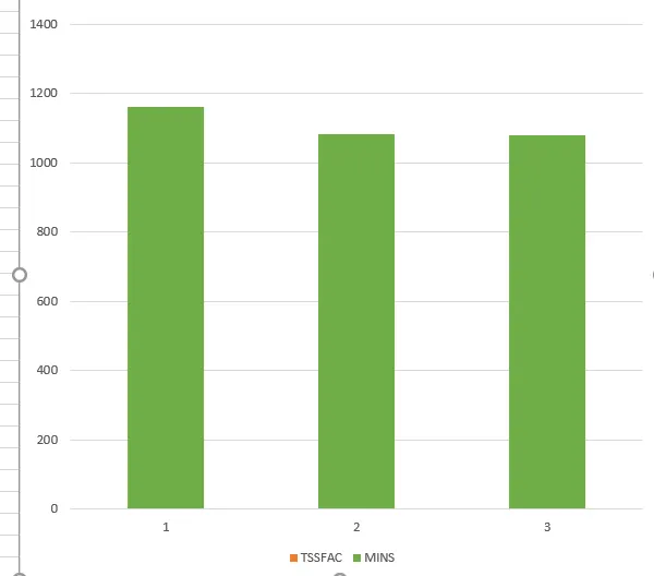
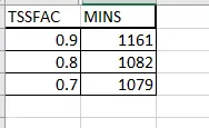
From the above plot i chossen the -6e-5 DT2MS value and TSSFAC values to 0.9, 0.8 and 0.7 you can see the time reuired to simulate decreses as TSSFAC value decreses

IMPLICIT ANALYSIS:

In implicit analysis implicit control cards are added i.e, CONTROL_IMPLICIT_GENERAL and CONTROL_IMPLICIT_AUTO

* CONTROL_IMPLICIT_GENERAL keyword is used to activate the implicit analysis by changing the IMFLAG value to 1

* CONTROL_IMPLICIT_AUTO keyword is used to activate the auto time step according to the requirement.

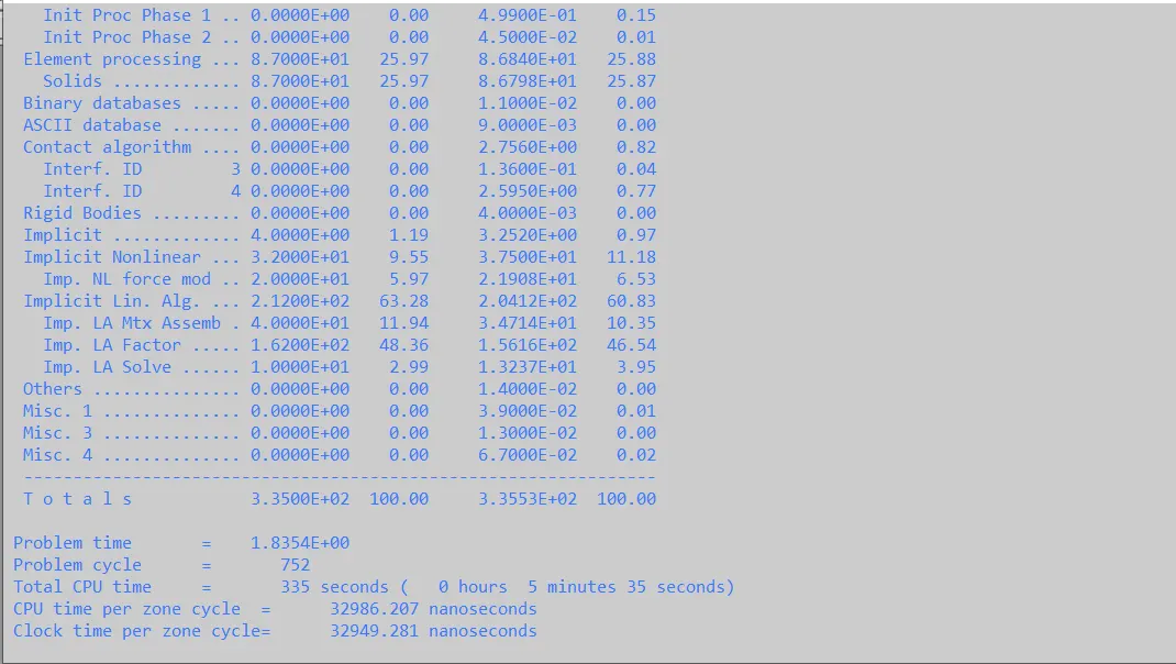
For implicit analysis it is not possible to predict the total time required to simulate. This is because implicit solver considers global equilibrium at each and every time step. also non linearity plays a major factor in the iteration involved since these values can be computed only at the time of the simulation it won't be possible to predict the value at the start of the simulation.

CONCLUSION :

As from the given objective the challenge is mainly focused on the getting the idea of mass scaling. From the above results we can see using mass scaling option we can reduce the run time but also we need to focus on mass percentage increase i.e, upto 8% to 10% above that the inertia of the model may changes to big value and it may cause the model to run in an in instable manner and results obtained may not satisfy the expectation. For implicit analysis, it won't be possible to compare with explicit analysis due to reasons mentioned in the report.