Week - 8 Mass Scaling
Mass Scaling:
Aim: Mass scaling to reduce the runtime of a model and ensure the stability of mass scaling. The hard limit on mass scaling is 8% and stability should be completely intact. This means that two simulations, one with mass scaling and one without should behave exactly the same way. The submission should contain the trials for mass scaling and the data generated henceforth. Both the DT2MS and TSSFAC parameters should be optimized, which are present under the Control-Timestep card.
All units used here are in kg,m,s which is decided depending upon the conversion factor in LS Dyna Challenge 1.
Steps followed:
Import the model provided in .k format with already having parts of Lower pin,Upper pin & plates,section of solid & meshing,Contacts,Controls & Databases as mentioned below:
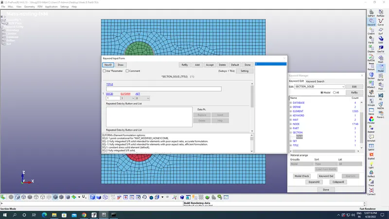
Section:
A section-solid is selected under keyword with Element formulation of 1 for constant stress solid element & appropriate section ID as shown in the image below:
Materials:
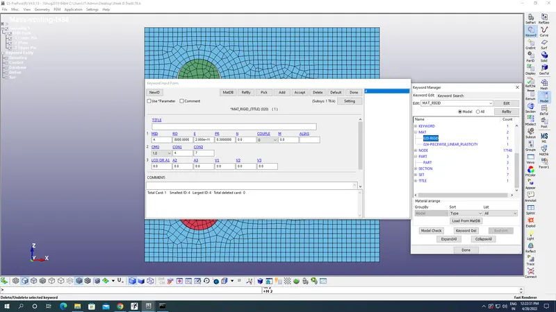
A rigid material of Mat 020 is defined for Upper & Lower pin which are of green & red color with material parameters of density,Young’s modulus & Poisson's ratio as shown in the image below:
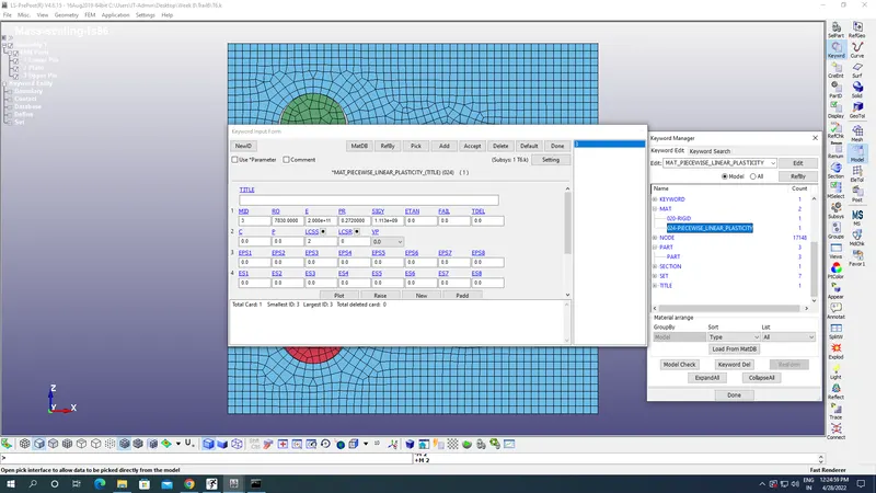
A Piecewise Linear Plastic material of Mat 024 s defined for Plate which is of blue color with material parameters of density 7830 kg/m^3,Young’s modulus 2E+11 kg mm^-1 ms^-2 & Poisson's ratio 0.27 & Yield stress 1.13E+09 kg mm^-1 ms^-2 as shown in the image below:
Parts:
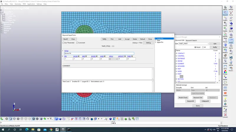
Go to Keyword option under Models & select parts with appropriate material ID,section ID,part ID & part title as shown in the images below:
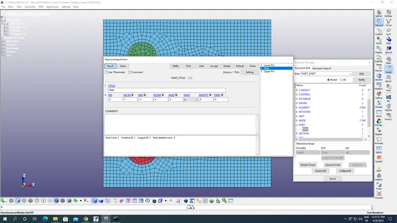
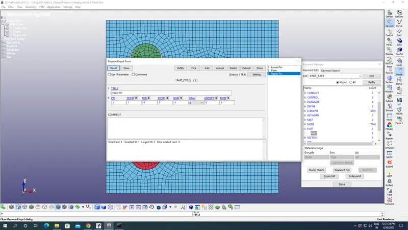
Set segments:
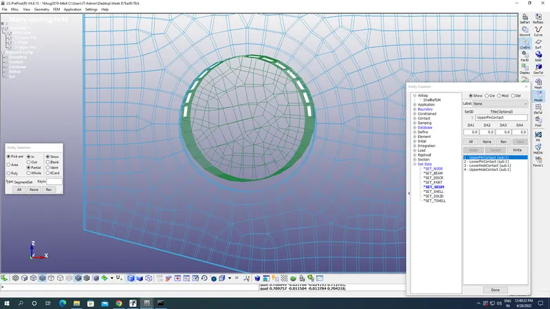
Four set segments are created for two Holes & Pins as shown in the image below:
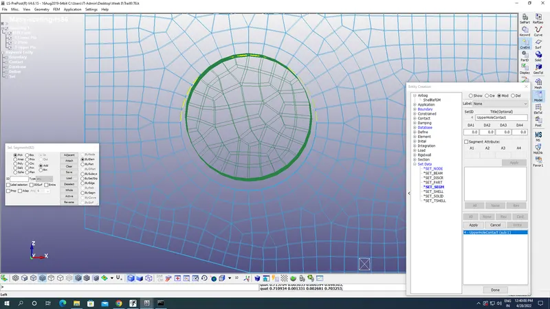
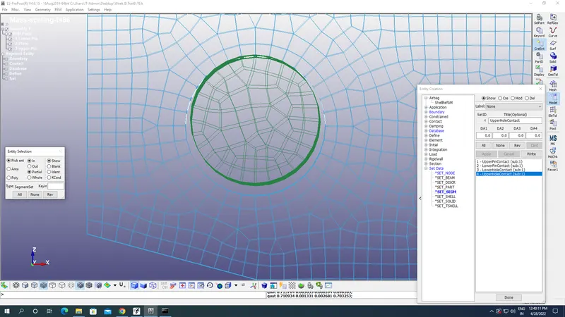
Contact surface:
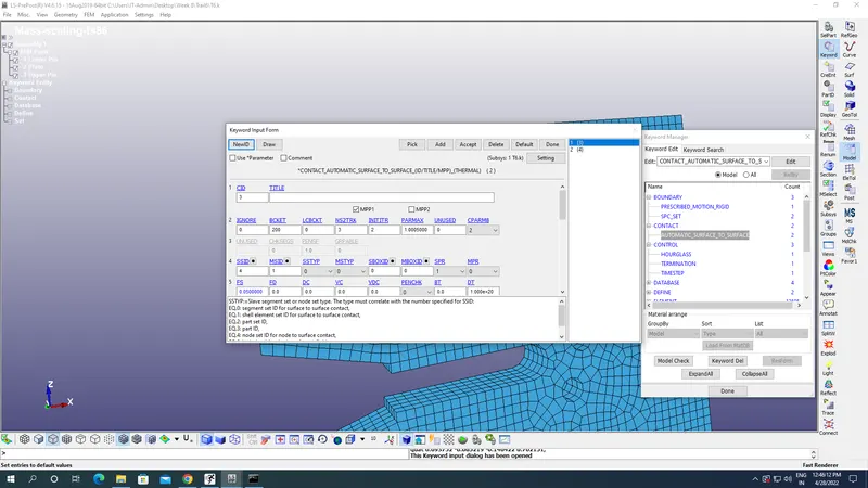
Now we are defining Automatic surface to surface contact by selecting set segments of master & slave sets by selecting Slave set type(SSTYP) And Master segement set type(MSSTYP) as 0 with proper set segment ID selection with Holes as slave & PIns as master as shown in the image below.
Boundary conditions:
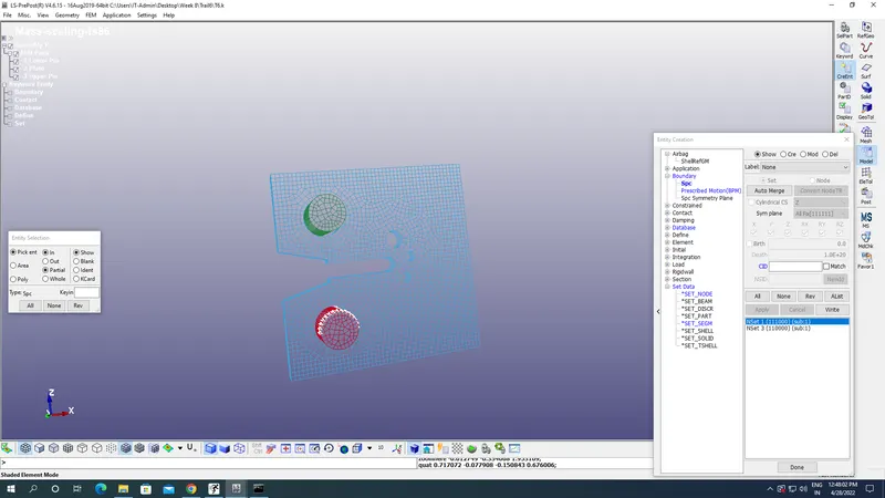
Now apply Single Point constrained(Spc) to the pins by going into create entity option under models Boundary-SPC in order to apply fixed boundary condition at the pins as shown in the image below:
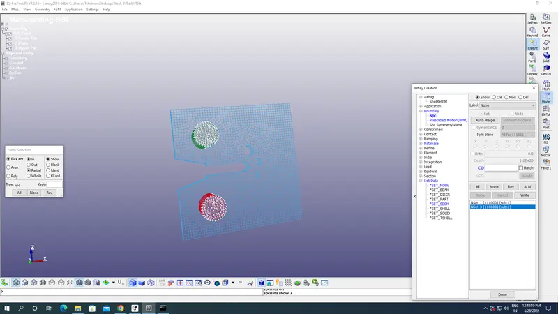
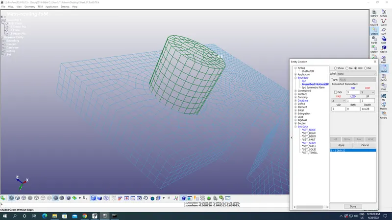
Apply Prescribed motion by going into create entity by selecting the elements of lower pin in green color as shown in the image with velocity as defined by Load curve id and Degree of Freedom(DOF) as 3 i.e translational along Z axis as shown in the image below:
Load Curves:
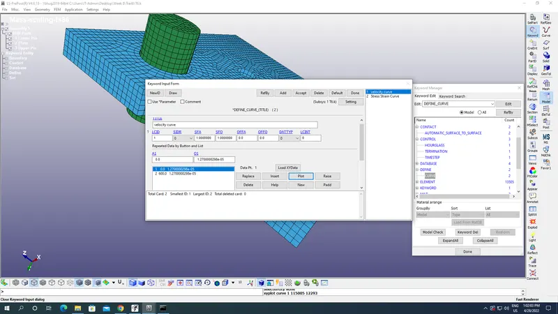
Go to Define-Curve under keyword option:
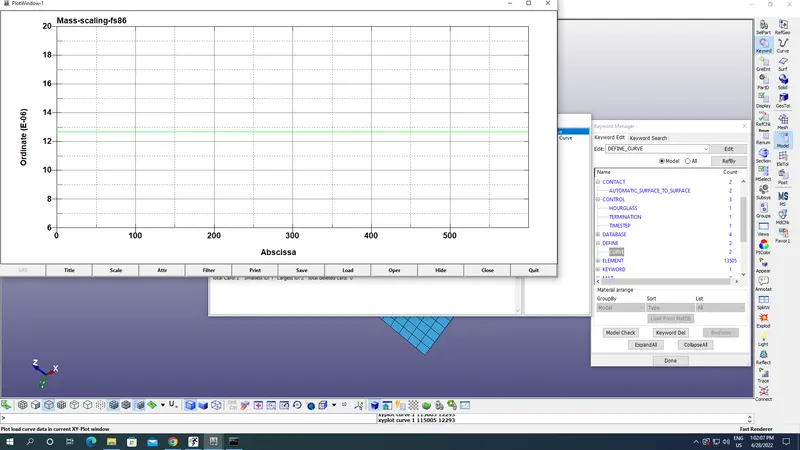
Load Curve for velocity:
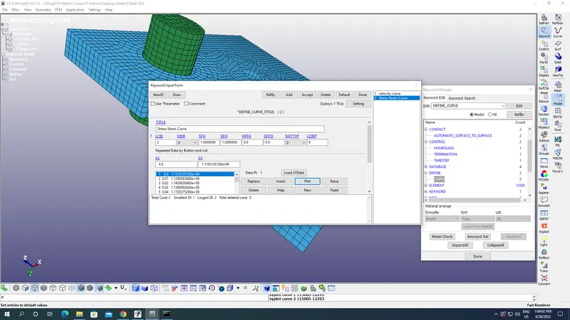
Load Curve for Stress-Strain:
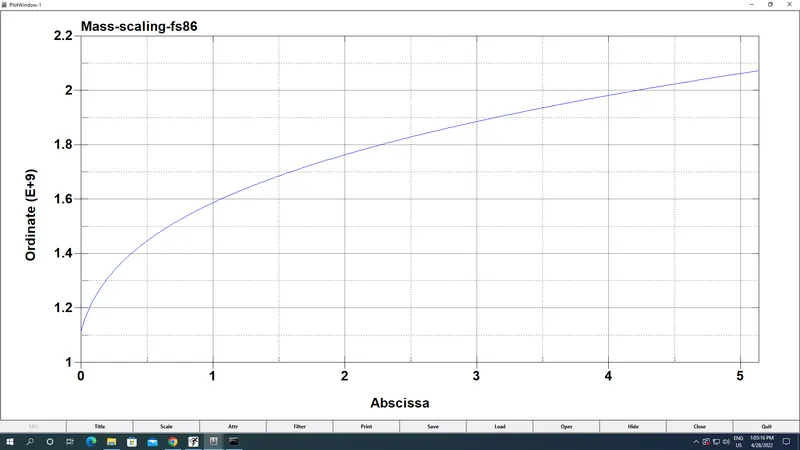
Controls:
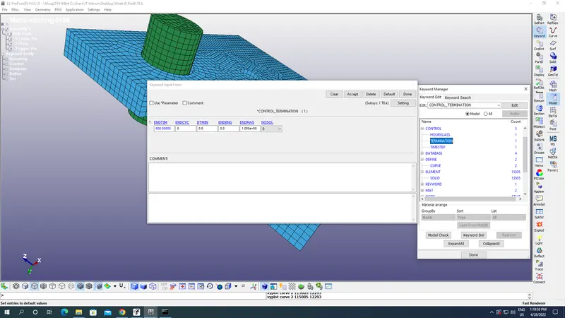
Now go to controls under keyword option and select the termination with End time as 600 s for the termination of simulation as shown in the image below:
Mass Scaling:
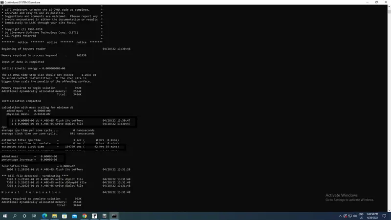
Mass scaling is used to reduce our run time during simulation because with Explicit solver actually the predetermined time step(dt) is very small for which it will take more time, like here Termination Time is 600 s but dt with DT2MS of -3.5E-05s is 4.40E-05 s
As shown in the image below due to which run time needed is 154799 s with zero added mass & mass addition percentage.
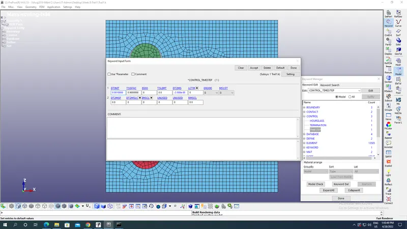
Under Controls go to Timestep for Structural Time step and define Initial time step size(DTINIT) as 0.001s with Time Scale Factor(TSSFAC) as 0.9,DT2MS(Time step for mass scaled solutions) as -7.8E-05s in order to add mass to decrease our Run time.Here negative sign indicates that mass scaling to occur due to which when DT2MS becomes greater than dt which is predetermined by the Double sparse solver as shown in the image below:
Case 1:
Trail 1:
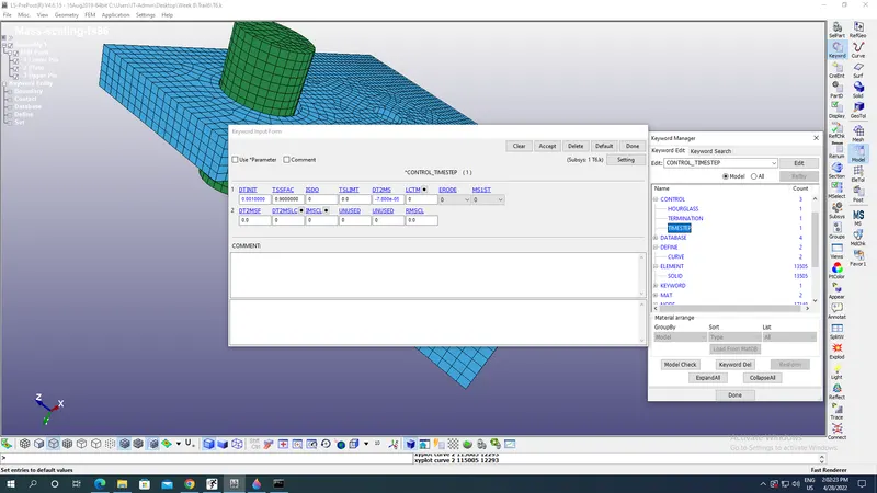
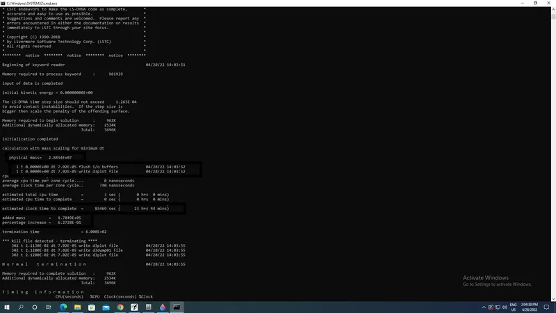
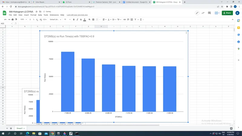
DT2MS=-7.8E-05s,TSSFAC=0.9 with dt 7.02E-05s,Physical mass=2.845E+07 kg,Mass added=1.78E+05 kg,Percentage of mass increase=0.627%,Total Run time=85472s.
Trail 2:
DT2MS=-8.80E-05 s,TSSFAC=0.9
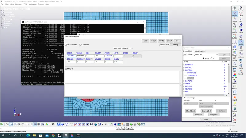
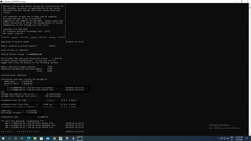
DT2MS=-8.8E-05s,TSSFAC=0.9 with dt 7.92E-05s,Physical mass=2.845E+07 kg,Mass added=6.34E+05 kg,Percentage of mass increase=2.23%,Total Run time=75760s.
Trail 3:
DT2MS=-9.80E-05 s,TSSFAC=0.9
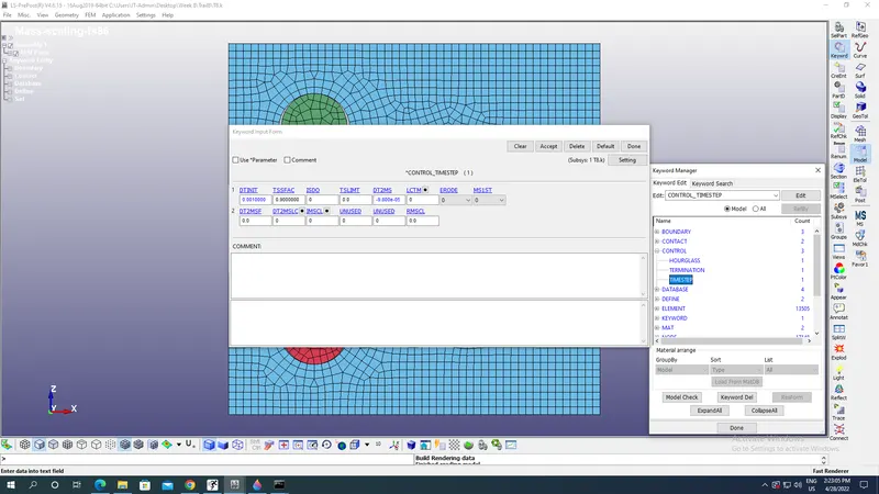
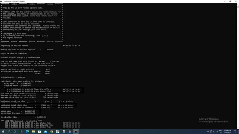
DT2MS=-9.8E-05s,TSSFAC=0.9 with dt 8.82E-05s,Physical mass=2.845E+07 kg,Mass added=1.56E+06 kg,Percentage of mass increase=5.49%,Total Run time=67411s.
Trail 4:
DT2MS=-1.01E-04 s,TSSFAC=0.9
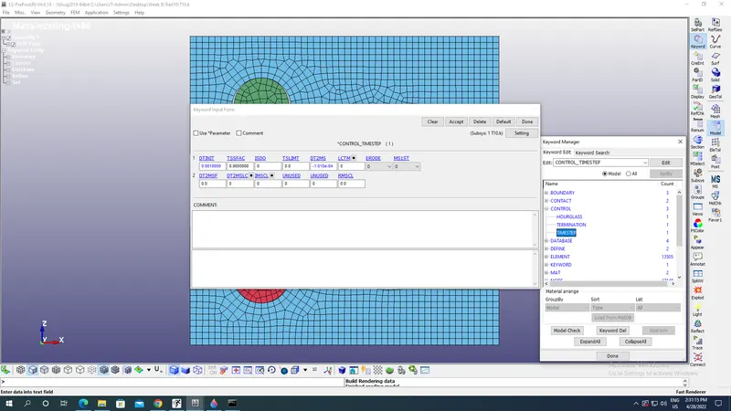
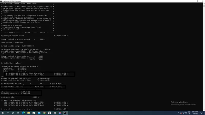
DT2MS=-1.01E-04s,TSSFAC=0.9 with dt 9.09E-05s,Physical mass=2.845E+07 kg,Mass added=1.97E+06 kg,Percentage of mass increase=6.9%,Total Run time=65409s.
Trail 5:
DT2MS=-1.02E-04 s,TSSFAC=0.9
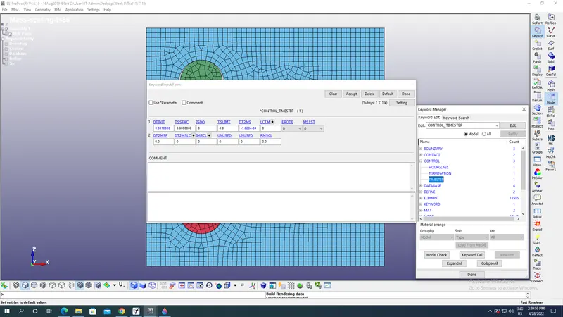
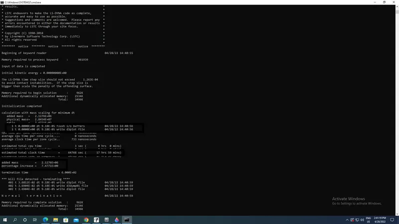
DT2MS=-1.02E-04s,TSSFAC=0.9 with dt 9.18E-05s,Physical mass=2.845E+07 kg,Mass added=2.13E+06 kg,Percentage of mass increase=7.47%,Total Run time=64768s.
Trail 6:
DT2MS=-1.03E-04 s,TSSFAC=0.9
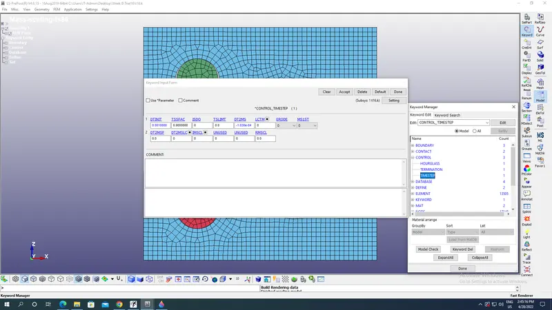
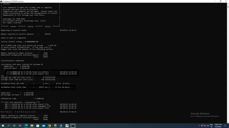
DT2MS=-1.02E-04s,TSSFAC=0.9 with dt 9.27E-05s,Physical mass=2.845E+07 kg,Mass added=2.29E+06 kg,Percentage of mass increase=8.06%,Total Run time=64727s.
So the permissible percentage of mass addition is 8% without any instability in the model during simulation.
Case2:
Similarly change Time scale factor (TSSFAC) 0.95 keeping the values of DT2MS same as in case1 so that the value of DT2M X SSFAC increase thereby decreasing our runtime compared to case1:
Trail 1:
DT2MS=-7.8E-05s,TSSFAC=0.95
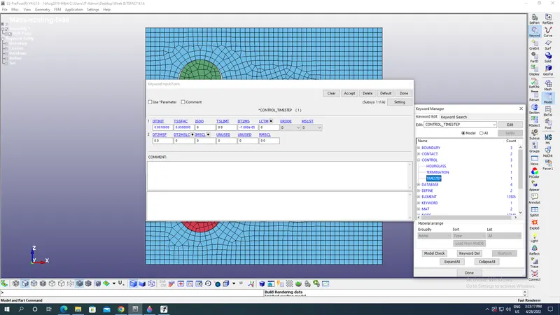
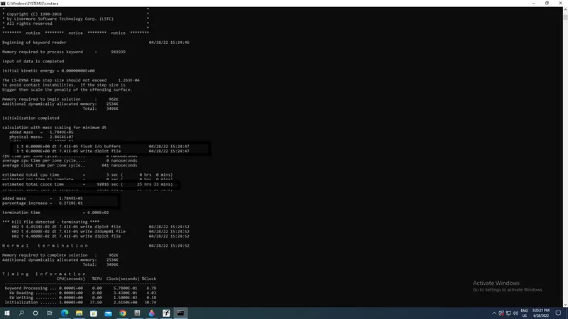
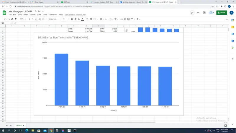
dt 7.41E-05s,Physical mass=2.845E+07 kg,Mass added=1.78E+05 kg,Percentage of mass increase=0.627%,Total Run time=82016s.
Trail 2:
DT2MS=-8.80E-05 s,TSSFAC=0.95
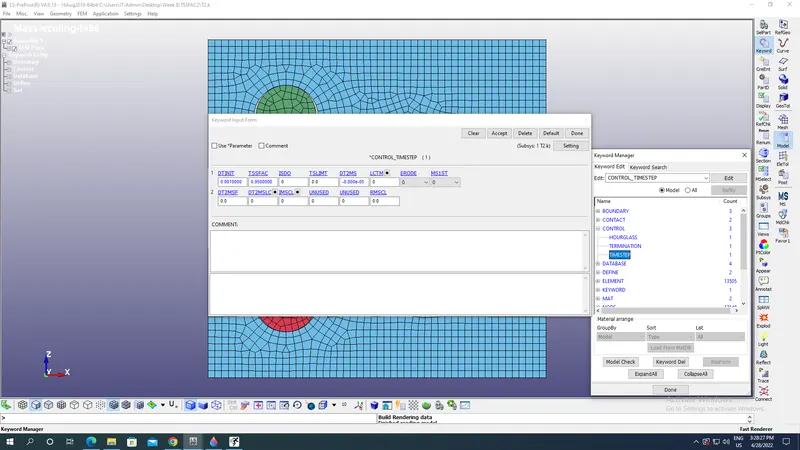
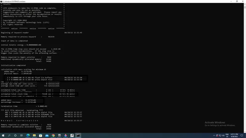
DT2MS=-8.8E-05s,TSSFAC=0.95 with dt 7.92E-05s,Physical mass=2.845E+07 kg,Mass added=6.34E+05 kg,Percentage of mass increase=2.23%,Total Run time=71120s.
Trail 3:
DT2MS=-9.80E-05 s,TSSFAC=0.95
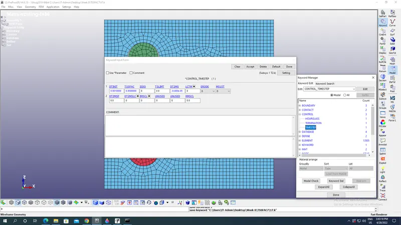
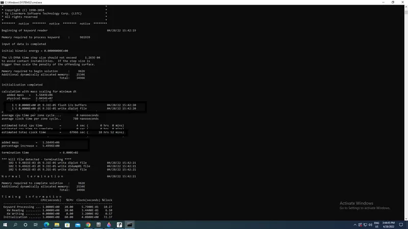
T2MS=-9.8E-05s,TSSFAC=0.95 with dt 9.31E-05s,Physical mass=2.845E+07 kg,Mass added=1.56E+06 kg,Percentage of mass increase=5.49%,Total Run time=67966s.
Trail 4:
DT2MS=-1.01E-04 s,TSSFAC=0.95
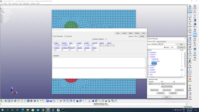
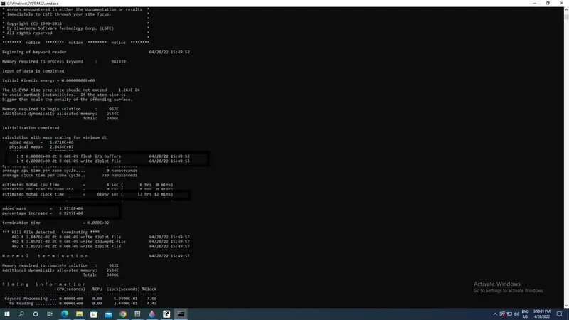
DT2MS=-1.01E-04s,TSSFAC=0.95 with dt 9.60E-05s,Physical mass=2.845E+07 kg,Mass added=1.97E+06 kg,Percentage of mass increase=6.9%,Total Run time=61967s.
Trail 5:
DT2MS=-1.02E-04 s,TSSFAC=0.95
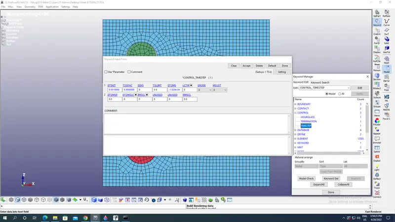
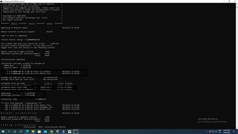
DT2MS=-1.02E-04s,TSSFAC=0.9 with dt 9.69E-05s,Physical mass=2.845E+07 kg,Mass added=2.13E+06 kg,Percentage of mass increase=7.47%,Total Run time=61922s.
Trail 6:
DT2MS=-1.03E-04 s,TSSFAC=0.9
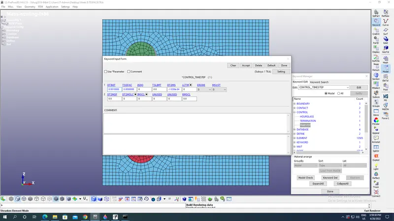
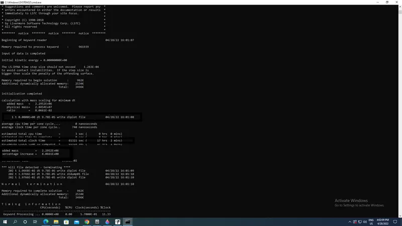
DT2MS=-1.02E-04s,TSSFAC=0.9 with dt 9.78E-05s,Physical mass=2.845E+07 kg,Mass added=2.29E+06 kg,Percentage of mass increase=8.06%,Total Run time=61321s.
So the permissible percentage of mass addition is 8% without any instability in the model during simulation.
Case 3:
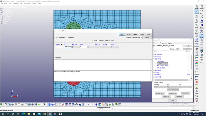
Now we are using implicit solver to find out our result so here we will delete timestep and within Control Implicit General card is applied with IMFLAG=1 for Implicit solver with DT0 as 10 s for initial time step size as shown in the image below:
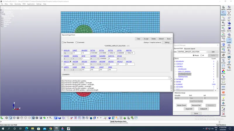
Now Control Implicit Solution is applied with NSOLV as 12 for Non linear implicit problem as shown in the image below:
All Termination,elements section remains same as in case 1 only Time step in Control is deleted because implicit solution does not depend on time.
Now we will run the file after saving it & final solution with runtime appears as shown:
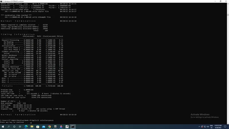
The run time seen from the image above is 173 s which is far less than Explicit solution time.
Results:
Plot of DT2MS vs Run time with TSSFAC as 0.9:
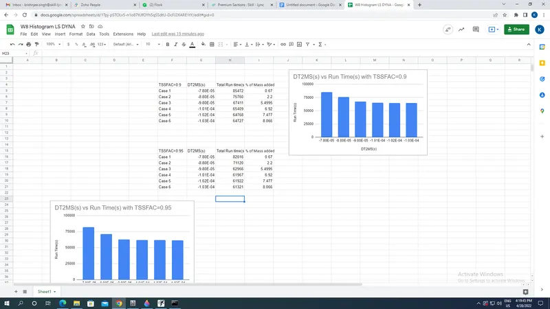
Plot of DT2MS vs Run time with TSSFAC as 0.95 with same values of DT2MS:
Run time for Implicit solver:
Comparison of cases with TSSFAC of 0.9 & 0.95:
From the Histogram plots above with DT2MS vs Run Time plot we can easily observe that RUN TIME after increase in TSSFAC from 0.9 to 0.95 decreases this occurs because with increasing TSSFAC the scale factor increases so the Time step which is compared with Solver dt as DT2M X SSFAC increases so it crosses dt easily resulting in mass scaling by same amount but at less run time.
Comparison between IMPLICIT & EXPLICIT Solvers Run time:
From the Run time images above we can see that time required for Implicit solver is less than explicit one because the Implicit solver takes longer steps which is very high compared to the dt steps taken by solver with Explicit one so Run time of Implicit is 2 minutes 30 seconds while that of explicit is about 20 to 50 hours.
Conclusion:
- Mass scaling is done upto 8% mass increase without causing instability in the model with scale factor as 0.9 & 0.95 with same mass scaling time by hit & trial method.
- The explicit & implicit run-time are compared with less time pf Implicit solver.