Week - 8 Mass Scaling

Understanding the implementation of Mass scaling using LS-Dyna

1. Introduction

Mass scaling is defined as a technique in FEA where non-physical mass is added in a structure to achieve a larger timestep size in explicit simulation. The step size is dependent on a number of factors including the size of the smallest elements. Usually smaller the element size, the smaller will be the time step size selected by the solver when using an explicit scheme. In larger problems, it can lead to an increase in runtime leading to high computation cost.

Mass scaling deals with this issue by adding and subtracting mass according to set criteria in the solver. In this exercise, a simple model containing a plate held by two rigid pins was given a very high termination time of 600 seconds so that its explicit simulation should be taking a very long time. Further, mass scaling was used to bring down the simulation time while keeping the percentage of added mass under 8%.

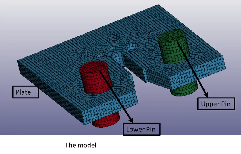
Fig 1.1: the geometry used for modelling the problem

The geometry in the model was meshed using solid elements (Hexa and tetra elements). Steel was assigned as material to the plate while a rigid material card was used for the pins. The aim of this exercise was to understand the implementation of mass scaling using the *control_timestep card in the LS-Dyna. Since we were not interested in the outcomes like stress-strain, the simulation runs in explicit solver were stopped after two steps taking note of the expected simulation time displayed in the message window.

2. Parameters used for mass scaling and their impact on the runtime

The control timestep card is used for controlling mass scaling in the model. There are two parameters namely DT2MS (time step size for mass scaling) and TSSFAC (time scale factor for mass scaling). DT2MS value specifies the timestep value for which mass scaling needs to be applied i.e. an element that leads to step size of that value will be added with mass. The TSSFAC value further scales the DT2MS value. The DT2MS value can be entered as a negative as well as a positive number.

Negative: Mass is added to only those elements whose timestep would otherwise be less than TSSF*abs(DT2MS). When mass scaling is appropriate, this method is recommended.

Positive: Mass is added or taken away from elements so that the timestep of every element is the same. There is no advantage to using this method over the negative DT2MS value. IN our case, the negative value approach was used.

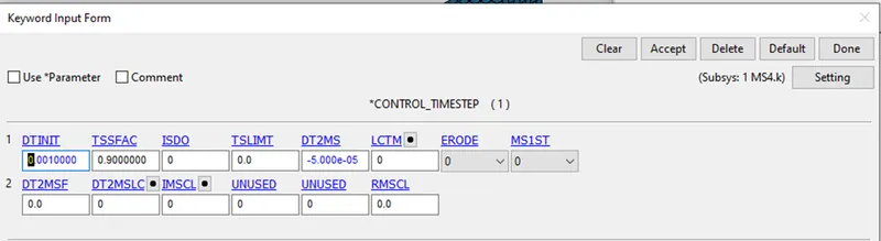
Fig 2.1: The control timestep card

Combinations of TSSFAC and DT2MS values were used to optimize the simulation time for explicit analysis of the model while keeping the added mass below 8%. In the following sections, they are discussed one by one.

2.1 The value of TSSFAC = 0.9 and DT2MS = -3.5e-5

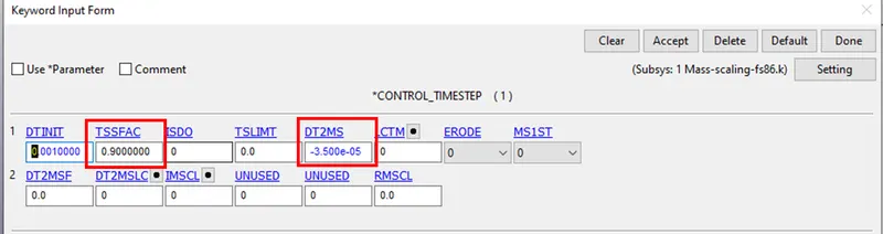
Fig 2.1: The control timstep card used for first iteration of the run time optimisation

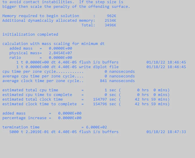
Fig 2.2: The message window showing an expected runtime of 42 hours and 59 minutes

This is a pretty high value of expected time to complete the simulation. Also, there is no apparent mass scaling happening as the added mass value is zero.

2.2 The value of TSSFAC = 0.7 and DT2MS = -3.5e-5

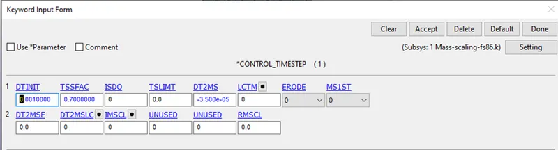
Fig 2.2: The control timstep card used for first iteration of the run time optimisation

Only the TSSFAC value was adjusted to 0.7 to see the effect.

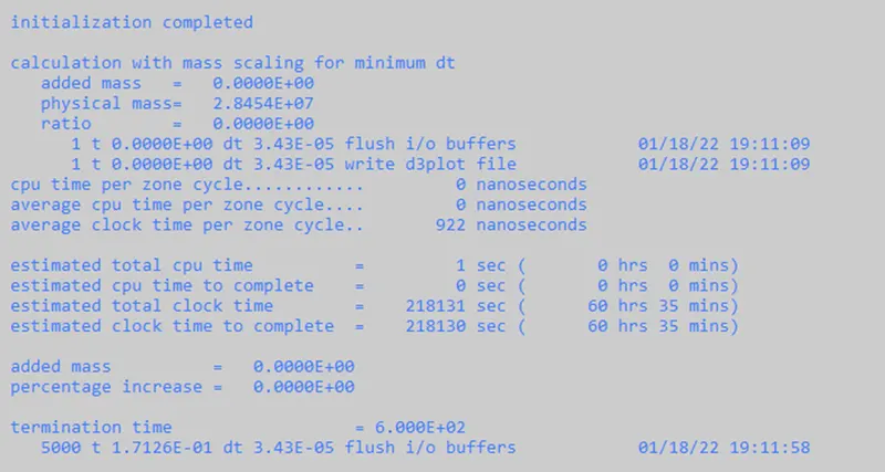
Fig 2.3: the message window showing the expected runtime for the settings

This is a whopping increase of almost 200%. To confirm this trend two more attempts were made by reducing the TSSFAC value as shown in the below-given table.

DT2MS	TSSFAC	Expected time
-3.5e-5	0.6	67 Hrs 35 Mins
-3.5e-5	0.5	83 Hrs 35 Mins

This confirms the fact that reduction in the TSSFAC value alone was having an adverse effect on the expected completion time of the simulation.

2.3 Altering the DT2MS value for optimisation of the expected completion time

The changed DT2MS value and the change in the expected time of completion are shown in the below-given table.

S.N.	DT2MS	TSSFAC	mass addition	Expected time	Inference
1	-5e-5	0.9	1.3179e-3%	47 Hrs 28 Mins	Time increased by 5 Hrs so need to increase DT2MS value
2	-1e-4	0.9	6.4233%	21 Hrs 2 Mins	Significant reduction in expected completion time
3	-1.1e-4	0.9	20.393%	19 Hrs 7 Mins	Added mass is more than 8%
4	-1e-4	0.7	6.4233%	30Hrs 18 Mins	TSSFAC value reduction has an adverse effect on expected time
5	-1e-4	0.6	6.4233%	35 Hrs 36 Mins	TSSFAC value reduction has an adverse effect on expected time
6	-1.05e-4	0.9	10.748%	20 Hrs 2 Mins	Added mass is more than 8%
7	-1.01e-4	0.9	6.9297%	23 Hrs 20 Mins	Further increase in DT2MS value has an adverse effect on expected time
8	-1.015e-4	0.9	7.198%	23 Hrs 23 Mins	Further increase in DT2MS value has an adverse effect on expected time
9	-1.02e-4	0.9	7.477%	23 Hrs 16 Mins	Further increase in DT2MS value has an adverse effect on expected time
10	-1.025e-4	0.9	7.766%	30 Hrs 52 Mins	Further increase in DT2MS value has an adverse effect on expected time

Table 2.3.1: The expected time obtained using various combinations of parameters

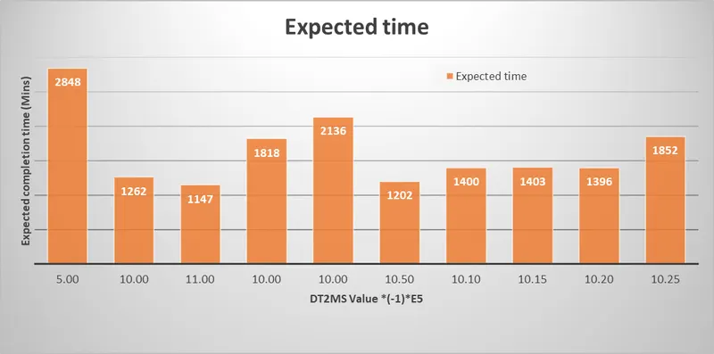
Chart 2.3.1: variation of expected completion time against DT2MS values

Conclusion: Clearly the best result is obtained using a TSSFAC=0.9 and DT2MS= -1e-4.

3. Simulation of the model using Implicit solver

The same model was run using the implicit scheme to see the time taken to complete the model. In an implicit scheme unlike the explicit method, there is no limitation on timestep size.

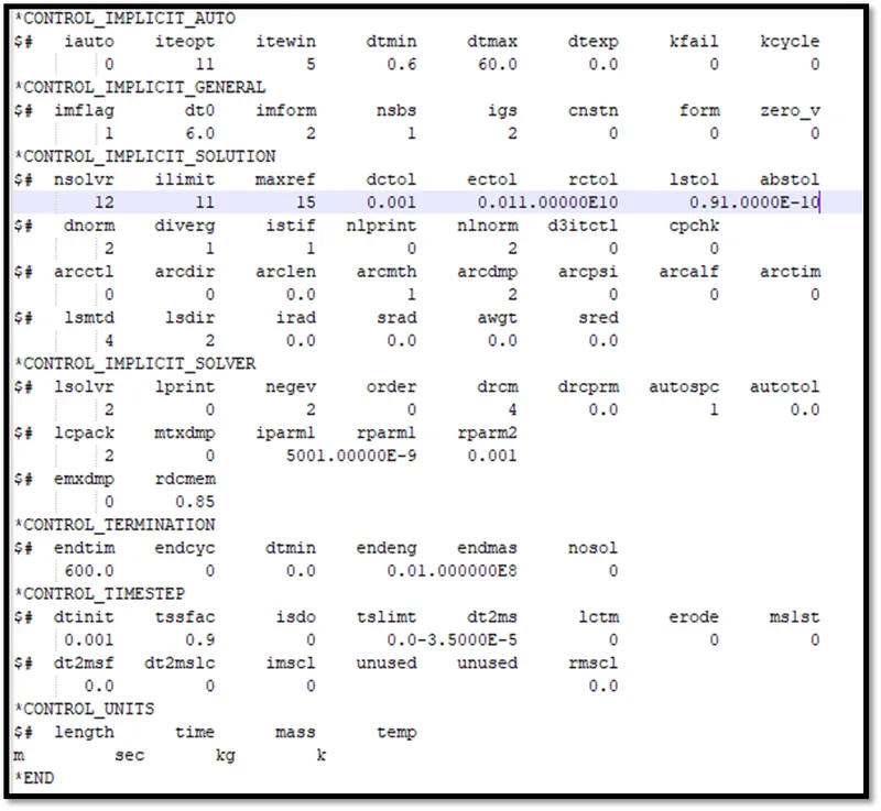
Fig 3.1: The implicit cards used for using the implicit solver

DT0 was kept to 6, DTMAX to 60 and the rest of the parameters were kept default. This was in accordance with the thumb rule of DT0= termination time/100.

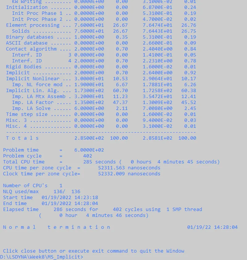
Fig 3.2: The message window showing the progress of solver in implicit mode

As clear from the above figure, the implicit scheme was very fast. It can be attributed to the fact that in the implicit scheme the concept of time is not exactly time. It can be thought of as load steps. Also, there is not any limitation on timestep size which enabled us to use up to 60 s for a single time step (it can go much higher).

Conclusion:

• Mass scaling plays a significant role in explicit simulations.
• A significant reduction in simulation time can be achieved using TSSFAC and DT2MS values