Week 8: Literature review - RANS derivation and analysis

AIM: To apply reynold's decomposition to the NS equations and come up with the expression for reynold's stress.

Introduction:

Navier stokes Equation:

Navier-Stokes equation, in fluid mechanics, a partial differential equation that describes the flow of incompressible fluids. The equation is a generalization of the equation devised by Swiss mathematician Leonhard Euler in the 18th century to describe the flow of incompressible and frictionless fluids.

The Navier–Stokes equations mathematically express conservation of momentum and conservation of mass for Newtonian fluids. They are sometimes accompanied by an equation of state relating pressure, temperature and density. They arise from applying Isaac Newton's second law to fluid motion, together with the assumption that the stress in the fluid is the sum of a diffusing viscous term (proportional to the gradient of velocity) and a pressure term—hence describing viscous flow.

The difference between them and the closely related Euler equations is that Navier–Stokes equations take viscosity into account while the Euler equations model only inviscid flow. As a result, the Navier–Stokes are a parabolic equation and therefore have better analytic properties, at the expense of having less mathematical structure.

Conservation of Mass:
The mass in the control volume can be neither be created nor destroyed. The conservation of mass states that the mass flow difference throughout the system between inlet and outlet is zero:

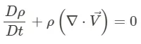where ρ is density, V is velocity and gradient operator ∇.

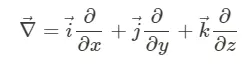
While the density is constant, the fluid is assumed incompressible and then continuity is simplified as below, which indicates a steady-state process:

Conservation of Momentum:

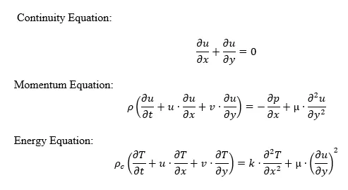
The momentum in a control volume is kept constant, which implies the conservation of momentum that we call ‘The Navier-Stokes Equations’. The description is set up in accordance with the expression of Newton’s Second Law of Motion:

Conservation of Energy:

Conservation of Energy is the first law of thermodynamics which states that the sum of the work and heat added to the system will result in the increase of the total energy of the system:

dEt=dQ+dW

where dQ is the heat added to the system, dW is the work done on the system, and dEt is the increment in the total energy of the system.

Turbulence:

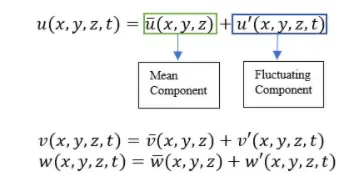
Turbulent flow can be applied to the Navier-Stokes equations to model the chaotic behavior. Apart from the laminar, transport quantities of the turbulent flow, it is driven by instantaneous values. Direct numerical simulation (DNS) is the approach to solving the N-S equations with instantaneous values. Having distinct fluctuations varying in a broad range, DNS needs enormous effort and expensive computational facilities. To avoid those hurdles, the instantaneous quantities are reinstated by the sum of their mean and fluctuating parts as follows:

where u, v, and w are velocity components and T is temperature.

Reynolds Average Navier Stokes(RANS):

The basic tool required for the derivation of the RANS equations from the instantaneous Navier–Stokes equations is the Reynolds decomposition.

Reynolds decomposition is a mathematical technique used to separate the expectation value of a quantity from its fluctuations. For example, for a quantity {\displaystyle u} the decomposition would be

where denotes the expectation value of and are the deviations from the expectation value.

The RANS equations are primarily used to describe turbulent flows. These equations can be used with approximations based on knowledge of the properties of flow turbulence to give approximate time-averaged solutions to the Navier–Stokes equations. For a stationary flow of an incompressible Newtonian fluid, these equations can be written in Einstein notation in Cartesian coordinates as:

in 3D flow:

u(x,y,z,t)=baru (x,y,z)+u^'(x,y,z,t)__Equation 1

v(x,y,z,t)=barv (x,y,z)+v^'(x,y,z,t)__ Equation 2

z(x,y,z,t)=barz (x,y,z)+z^'(x,y,z,t)__ Equation 3

Time average quantities:

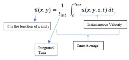
The momentary velocity components is u , the time-averaged value is named u and the fluctuating
velocity has the letter u′ . With help of this definition the decomposition can mathematically be written
as:
u = u + u′ , v = v + v′ , w = w + w′ , p = p + p′

for the density and the temperature:
ρ=ρ +ρ′ , T=T +T′ ,

which will however be considered constant in the following.

The chosen averaging method takes the mean values at a fix place in space and averaged over a time
span that is large enough for the mean values to be independent of it.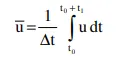

The time-averaged values of the fluctuating values are defined to be zero:
u′ = ,0 v′= ,0 w′= ,0 p′=0

Firstly the continuity equation is averaged.

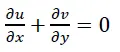
Applying the Reynold’s decomposition to the continuity equation:

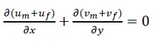
Integrating over the time interval:

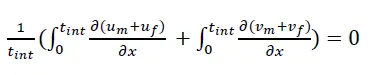
Now we can split the integrals as

We know that the integral of the fluctuating component is zero, hence:

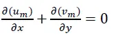
which is nothing but

Thus, the continuity equation can be simplified as:

Momentum Equation:

The momentum equation after neglecting few terms

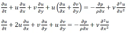
Taking the density term to the other side we get:

Adding the continuity equation multiplied by the x-component velocity on the right-hand side (since the continuity equation is 0 adding a term is permissible):

Now using the relation:

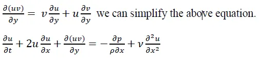
This can be further simplified into:

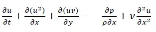
Now by applying time integration and Reynold’s Decomposition.

By splitting the integrals, we get:

Now by neglecting the integrals of fluctuating terms and by time integrating the rest of the terms we get the equation:

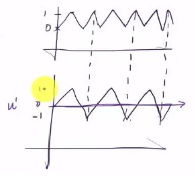
A graph of the fluctuating velocity 𝑢𝑓 can be seen in the image above. Since it oscillates between positive and negative values the average of it can be taken as zero and hence the time integral of 𝑢𝑓is zero.

But the square of its value is purely a positive one and hence the time integral of 𝑢𝑓2 is not zero.

Thus, we have the two negative time integral time on the right-hand side. Inside the boundary layer the change in velocity across the x-axis, i.e. the velocity gradient, is not as large as the y-axis and hence the square of x-velocity can be taken as zero. Using this assumption and by simplifying the equation:

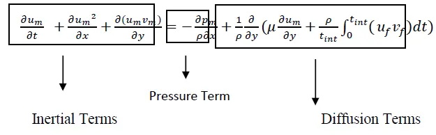
The diffusion terms primarily deal with how the momentum can be diffused. And momentum can be diffused in two ways:

1. Molecular Viscosity, i.e. also called viscous stress

2. Momentum diffusivity due to turbulent flow, i.e. 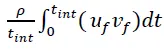also called Reynolds stress. The equation give above is the final expression for the Reynolds Averaged Navier Stokes equation and the only unknown term is the Reynolds Stress. As stated earlier, the primary aim of turbulence modelling is to capture the Reynolds Stress.

Turbulent Viscosity:

The turbulent transfer of momentum by eddies giving rise to an internal fluid friction, in a manner analogous to the action of molecular viscosity in laminar flow, but taking place on a much larger scale.

The value of the coefficient of eddy viscosity (an exchange coefficient) is of the order of 1 m2 s-1, or one hundred thousand times the molecular kinematic viscosity.

Eddy viscosity is often represented by the symbol K, and the turbulence parameterization that uses eddy viscosity is called K-theory. In this theory, the eddy flux in kinematic units is related to the mean vertical gradient. Since the turbulent viscosity K is the quantity being modelled the turbulence models have K- as the prefix. In general, molecular viscosity or viscosity is a fluid property. It is the measure of its resistance to gradual deformation by shear or tensile stress. It can be construed like some sort of internal friction between two layers of the fluid developed while flowing.

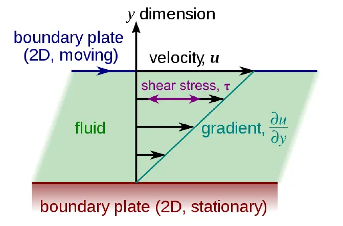
A symbolic representation of fluid flow over a boundary plate is as shown above. The gradient is nothing but velocity gradient arising within the fluid layers due to the friction acting between them. The magnitude of the shear stress is given by Newton’s law of viscosity is:

𝜏=𝜇*𝜕𝑢/𝜕𝑦

𝜇 is the coefficient of molecular viscosity. There are two different types of viscosity: Dynamic Viscosity and Kinematic Viscosity. The difference is based on the way in which viscosity is measured. One way is to measure a fluid’s resistance to flow when an external force is applied. This is dynamic viscosity.

Reynolds Stress:

The mean forces (per unit area) imposed on the mean flow by turbulent fluctuations.
They arise from the nonlinear advection term when the Navier–Stokes equations are Reynolds decomposed and Reynolds averaged. The general form of the Reynolds stress tensor is:

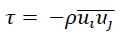
can be taken as the momentum dissipation in the x and y direction.
𝜏 is the Reynold’s Stress and 𝜌 is the density.

RNG K-epsilon Model:

The RNG model was developed using Re-Normalisation Group (RNG) methods by Yakhot et al to renormalize the Navier-Stokes equations, to account for the effects of smaller scales of motion.

In the standard k-epsilon model the eddy viscosity is determined from a single turbulence length scale, so the calculated turbulent diffusion is that which occurs only at the specified scale, whereas in reality all scales of motion will contribute to the turbulent diffusion.

The RNG approach, which is a mathematical technique that can be used to derive a turbulence model similar to the k-epsilon, results in a modified form of the epsilon equation which attempts to account for the different scales of motion through changes to the production term.