Week 8: Literature review - RANS derivation and analysis
Aim: -Literature review - RANS derivation and analysis
objectie:
Apply reynold's decomposition to the NS equations and come up with the expression for reynold's stress.
- Explain your understanding of the terms reynold's stress
- What is turbulent viscosity? How is it different from molecular viscosity?
theory:
reynolds number: is the ratio of inertial forces to viscous forces.
Reynolds number is a dimensionless quantity that is used to determine the type of flow pattern as laminar or turbulent while flowing.
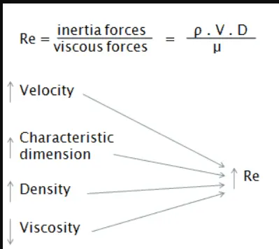
reynolds number calculation
Critical Reynolds Number for Flow in a Pipe
For flow in a pipe of diameter D, experimental observations show that for “fully developed” flow, the critical Reynolds number is about Red,crit = 2300.
- Laminar flow. For practical purposes, if the Reynolds number is less than 2000, the flow is laminar. The accepted transition Reynolds number for flow in a circular pipe is Red,crit = 2300.
- Transitional flow. At Reynolds numbers between about 2000 and 4000 the flow is unstable as a result of the onset of turbulence. These flows are sometimes referred to as transitional flows.
- Turbulent flow. If the Reynolds number is greater than 3500, the flow is turbulent.
Critical Reynolds Number in boundary layer flow over a flat plate.
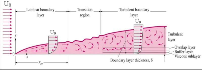
flow region and boundary layer on a flat plate
uo is free stream velocity it is out side the boundary layer and in side boundary layer the velocity is changing along y direction
Turnulence modeling
Turbulence modeling is the construction and use of a mathematical model to predict the effects of turbulence.
these model used beacause
Because the smallest scales of turbulence are very large compared to molecular dimensions, turbulence is a continuum phenomenon. Consequently, the Navier-Stokes, energy and mass-conservation equations contain all of the physics of turbulent fluid motion. However, even with the power of computers at the beginning of the twenty-first century, exact numerical simulations remain practicable only at low Reynolds numbers.
Since exact turbulent-flow solutions are so computationally extensive, we use models to achieve practical computation times. We pay a price for this convenience, of course, because a model approximates the exact equations of motion. By their nature, turbulence models are based mainly on dimensional analysis combined with intuition and experimental observations. Given such a tenuous foundation, their range of applicability can only be ascertained by numerous comparisons with measurements for carefully documented flows.
Reynolds-averaged Navier–Stokes equations (RANS equations)
The Reynolds-averaged Navier–Stokes equations (RANS equations) are time-averaged equations of motion for fluid flow. The idea behind the equations is Reynold’s decomposition, whereby an instantaneous quantity is decomposed into its time-averaged and fluctuating quantities, an idea first proposed by Osborne Reynolds. The RANS equations are primarily used to describe turbulent flows. These equations can be used with approximations based on knowledge of the properties of flow turbulence to give approximate time-averaged solutions to the Navier–Stokes equations.
Reynolds decomposition
Reynolds decomposition is a mathematical technique used to separate the expectation value of a quantity from its fluctuations.
governing eqn for the boundary layer(Navier–Stokes equations)
`(du)/dx+(dv)/dy=0` --> continuety eqn
`rho((du)/dt+u*(du)/dx+v(du)/dy)=-(dp)/dx+mu(d^2u)/dy^2` --> mommentum eqn
`rho*C_p((dT)/dt+u(dT)/dx+v(dT)/dy)=K(d^2T)/dx^2+mu((du)/dy)^2`--> energy eqn
renolds decomposition
`u(x,y,z,t)=bar(u)(x,y,z)+u'(x,y,z,t)`
`bar(u)(x,y,z)-`time average quqntity
u'(x,y,z,t)- flucatuating quqntity
here
`1/t*int_0^tu'(x,y,z,t)=0`-->(1) [ fluctuation quantity time avrge is equal to 0]
continuety eqn
`(du)/dx+(dv)/dy=0`
reynolds decomposiion
`d/dx*(bar(u)+u')+d/dy(bar(v)+v')=0`
inigration wrt time
`1/tint_0^t[(d/dx(bar(u))+d/dx(u')+d/dy(bar(v))+d/dy(v')]dt=0`
from eqn 1 wkt fluctuation quantity wtr tp time is equal to 0
now simplifing the eqn we get
`1/tint_0^t[(d/dx(bar(u))+d/dy(bar(v))]dt=0`
`d/dx(bar(u)) & d/dy(bar(v))` are time indepedent so they take outside
`d/dx(bar(u))(t-0)/t+d/dy(bar(v))*(t-0)/t=0`
`d/dx(bar(u))+d/dy(bar(v))=0`
the above eqn is same as contuinuety eqn but this is time arged eqn
mommentum eqn
`rho((du)/dt+u*(du)/dx+v(du)/dy)=-(dp)/dx+mu(d^2u)/dy^2`
divide by `rho` on both side
`((du)/dt+u*(du)/dx+v(du)/dy)=-1/rho*(dp)/dx+mu/rho*(d^2u)/dy^2`
wkt `mu/rho=nu`
`((du)/dt+u*(du)/dx+v(du)/dy)=-1/rho*(dp)/dx+nu*(d^2u)/dy^2`
add continuety eqn to above eqn
`((du)/dt+u*(du)/dx+v(du)/dy)+u*((du)/dx+(dv)/dy)=-1/rho*(dp)/dx+mu/rho*(d^2u)/dy^2`
`(du)/dt+2*u*(du)/dx+v(du)/dy+u*(dv)/dy=-1/rho*(dp)/dx+mu/rho*(d^2u)/dy^2`
`(du)/dt+2*u*(du)/dx+d/dy(u*v)=-1/rho*(dp)/dx+mu/rho*(d^2u)/dy^2`
`because v(du)/dy+u*(dv)/dy=d/dy(uv)`
further simplified
`(du)/dt+(du^2)/dx+d/dy(u*v)=-1/rho*(dp)/dx+mu/rho*(d^2u)/dy^2`
now apply demoposition
`d/dt(bar(u)+u')+d/dx((bar(u)+u'))^2+d/dy*((bar(u)+u')*(bar(v)+v'))=-1/rho*d/dx(bar(p)+p')+nu*(d^2((bar(u)+u'))/dy^2)`
aftrer smilifing
`d/dt(bar(u))+d/dt(u')+d/dx(bar(u))^2+d/dx(u')^2+d/dx(2*bar(u)*u')+d/dy(bar(u)*bar(v))+d/dy(bar(u)*v')+d/dy(u'*bar(v))=-1/rho*(d/dx(bar(p))+d/dx(p'))+nu(d^2/dy^2(bar(u))+d^2/dy^2(u'))`
inetegartion wrt time
`1/tint_0^t[d/dt(bar(u))+d/dt(u')+d/dx(bar(u))^2+d/dx(u')^2+d/dx(2*bar(u)*u')+d/dy(bar(u)*bar(v))+d/dy(bar(u)*v')+d/dy(u'*bar(v))]dt=-1/t*int_0^t[1/rho*(d/dx(bar(p))+d/dx(p'))+nu(d^2/dy^2(bar(u))+d^2/dy^2(u'))]dt`
using eqn (1) simplified
time integral these equal to zero
`d/dt(u')=d/dx(2*bar(u)*u')=d/dy(bar(u)*v')=d/dy(bar(v)*u')=d/dx(p')=d^2/dy^2(u')=0`
now
`1/t*int_0^t[d/dt(bar(u))+d/dx(bar(u)^2)+d/dy(bar(u)*bar(v))]dt=1/t*int_0^t[-1/rho*d/dx(bar(p))+nu(d^2/dy^2(bar(u)))-d/dx(u')^2-d/dy(u'*v')]dt`
wkt time integral of mean quantity is insipedent of time hence
`d/dt(bar(u))+d/dx(bar(u)^2)+d/dy(bar(u)*bar(v))=-1/rho*d/dx(bar(p))+nu*(d^2/dy^2(bar(u)))-1/t*int_0^td/dx(u')^2*dt-1/t*int_0^td/dy(u'v')*dt`
under boundary layer fluctuation along x direction is less
hence `1/t*int_0^td/dx(u')^2*dt=0`
final eqn
`d/dt(bar(u))+d/dx(bar(u)^2)+d/dy(bar(u)*bar(v))=-1/rho*d/dx(bar(p))+1/rho*d/dy[(mu*d/dy(bar(u)))-rho/t*int_0^t(u'v')*dt]`
here
`d/dt(bar(u))+d/dx(bar(u)^2)+d/dy(bar(u)*bar(v))`--> inertial term
`-1/rho*d/dx(bar(p))`-->pressure term
`mud/dy(bar(u))`--> molecular viscosity
`rho/t*int_0^t(u'v')*dt`--> momment of diffucivity of turbulence/raynolds stress
Reynolds stress
the Reynolds stress is the component of the total stress tensor in a fluid obtained from the averaging operation over the Navier–Stokes equations to account for turbulent fluctuations in fluid momentum.
`rho/t*int_0^t(u'v')*dt`--> momment of diffucivity of turbulence/raynolds stress
turbulent viscosity
In a turbulent flow, the mechanism of transverse momentum transport is dominated by bulk mixing at scales mostly well above the mean free path. So the effective viscosity in a region such as a turbulent boundary layer is much higher than in laminar flow. The more effective momentum transport due to the mixing in the turbulent boundary layer results in a thinner boundary layer between any wall in contact with the fluid and the free stream outside the boundary layer where the flow obeys potential flow laws.
molecular viscosity
Viscosity is the phenomenon (and the measure) of transverse momentum transport a moving fluid. In laminar flow the mechanism of momentum transport is diffusion due to molecular motion and the resutlting molecular collisions, the same as for mass transport and for heat conduction.
conclusion
by applying reynolds decomposition to the navior stokes eqn the renolds stress eqn is derived.