Project 2 - Rankine cycle Simulator

clear all 
close all
clc

disp('1-2 is isentropic expansion');
disp('2-3 is constant pressure heat rejection');
disp('3-4 is isentropic compression');
disp('4-1 is constant presure heat addion');
p1=input('enter the presure  at inlet of turbine=');%presure at inlet of turbine in bar

t1=input('enter the temprature at inlet of turbine=');% temprature at inlet of the turbine in degree celcius

p2=input('enter the presure outlet of turbine=');% presure at outlet of the turbine or inlet at condenser in bar
% state-1 

h_1=XSteam('h_PT',p1,t1);
s_1=XSteam('s_PT',p1,t1);

%state -2
s_2=s_1;%the expansio is isentropic expansion
t2=XSteam('tsat_p',p2);
s_2f=XSteam('sL_P',p2);
s_2g=XSteam('sV_P',p2);
x=(s_2-s_2f)/(s_2g-s_2f);
h_2=XSteam('h_Px',p2,x);

%state-3
p3=p2;
s_3=XSteam('sL_p',p2);
t3=t2;
h_3=XSteam('hL_p',p2);
v_3=XSteam('vL_p',p2);
wp=v_3*(p2-p1)*100;%work done on water to pump from p1 to p2


% state-4
p4=p1;
s_4=s_3;
cv4=XSteam('Cv_ps',p1,s_4);
cp4=XSteam('Cp_ps',p1,s_4);
k=cp4/cv4;

h_4=h_3+wp;
t4=t3/((p3/p4)^((k-1)/k));
wt=h_1-h_2;% work done by steam in turbine expansion process


%to find stauration liquid and vapour stete point
t5=XSteam('tsat_p',p1);
t6=t5;
s_5=XSteam('sL_p',p1);
h_5=XSteam('hL_p',p1);
s_6=XSteam('sV_p',p1);
h_6=XSteam('hV_p',p1);
t=linspace(1,375,1000);

%find efficiency, net work, back work done ,heat suplied and heat rejected  by rankine cycle

wp=v_3*(p1-p2)*100;%work done on water to pump from p1 to p2

wt=h_1-h_2;% work done by steam in turbine expansion process

wnet=wt-wp;%net wrk is diffrence b/w work done by water and on water
wb=wp/wt;%back work ratio is the ratio b/w -ve work to the +ve work
q_in=h_1-h_4;
q_rej=h_2-h_3;
eff=wt*100/q_in;

for i=1:length(t)
    sf(i)=XSteam('sL_T',t(i));
    sg(i)=XSteam('sV_T',t(i));
    hf(i)=XSteam('hL_T',t(i));
    hg(i)=XSteam('hV_T',t(i));
end
%to plot t-s diagram of rankine cycle
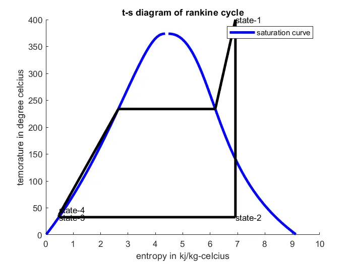
figure(1)
hold on

plot(sf,t,'b','linewidth',3)
plot(sg,t,'b','linewidth',3)
plot([s_1,s_2],[t1,t2],'k','linewidth',3)
plot([s_2,s_3],[t2,t3],'k','linewidth',3)
plot([s_3,s_4],[t3,t4],'k','linewidth',3)
plot([s_4,s_5],[t4,t5],'k','linewidth',3)
plot([s_6,s_5],[t6,t5],'k','linewidth',3)
plot([s_6,s_1],[t6,t1],'k','linewidth',3)
text(s_1,t1,'state-1');
text(s_2,t2,'state-2');
text(s_3,t3,'state-3');
text(s_4,t4+10,'state-4');
title('t-s diagram of rankine cycle')
xlabel('entropy in kj/kg-celcius')
ylabel('temorature in degree celcius')
legend('saturation curve')
hold off

% to plot the h-s diagram of rankine cycle
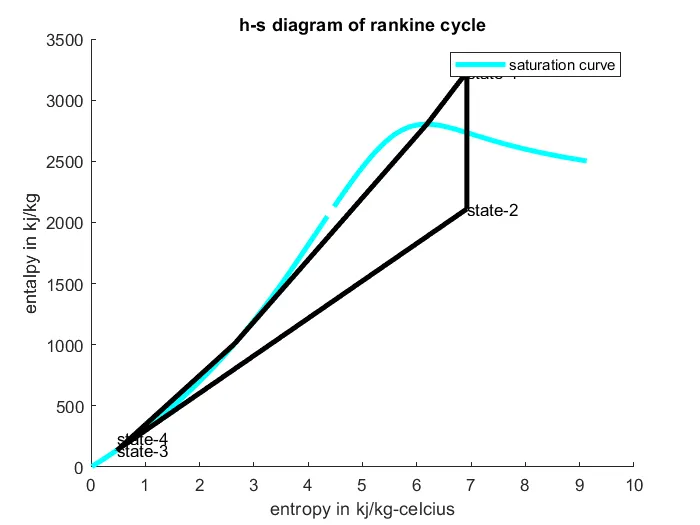
figure(2)
hold on
plot(sf,hf,'c','linewidth',3)
plot(sg,hg,'c','linewidth',3)
plot([s_1,s_2],[h_1,h_2],'k','linewidth',3)
plot([s_2,s_3],[h_2,h_3],'k','linewidth',3)
plot([s_3,s_4],[h_3,h_4],'k','linewidth',3)
plot([s_4,s_5],[h_4,h_5],'k','linewidth',3)
plot([s_6,s_5],[h_6,h_5],'k','linewidth',3)
plot([s_6,s_1],[h_6,h_1],'k','linewidth',3)
text(s_1,h_1,'state-1');
text(s_2,h_2,'state-2');
text(s_3,h_3,'state-3');
text(s_4,h_4+100,'state-4');
title('h-s diagram of rankine cycle')
xlabel('entropy in kj/kg-celcius')
ylabel('entalpy in kj/kg')
legend('saturation curve')
hold off
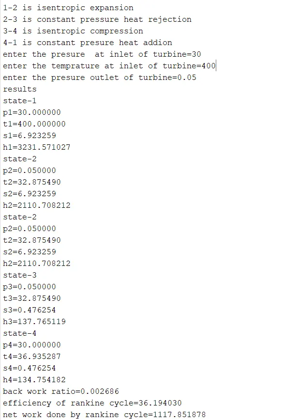
disp('results')
% state-1 variables
disp('state-1');
fprintf('p1=%4f\n',p1);
fprintf('t1=%4f\n',t1);
fprintf('s1=%4f\n',s_1);
fprintf('h1=%4f\n',h_1);

% state-2 variables
disp('state-2');
fprintf('p2=%4f\n',p2);
fprintf('t2=%4f\n',t2);
fprintf('s2=%4f\n',s_2);
fprintf('h2=%4f\n',h_2);

% state-2 variables
disp('state-2');
fprintf('p2=%4f\n',p2);
fprintf('t2=%4f\n',t2);
fprintf('s2=%4f\n',s_2);
fprintf('h2=%4f\n',h_2);
% state-3 variables
disp('state-3');
fprintf('p3=%4f\n',p3);
fprintf('t3=%4f\n',t3);
fprintf('s3=%4f\n',s_3);
fprintf('h3=%4f\n',h_3);

% state-4 variables
disp('state-4');
fprintf('p4=%4f\n',p4);
fprintf('t4=%4f\n',t4);
fprintf('s4=%4f\n',s_4);
fprintf('h4=%4f\n',h_4);


fprintf('back work ratio=%f\n',wb);
fprintf('efficiency of rankine cycle=%f\n',eff);
fprintf('net work done by rankine cycle=%f\n',wnet);

Aim:-
1.create rankine cycle simulation using matlab
2.calculate all state points of rankine cycle using XSteam function
3.plot t-s and h-s diagram of rankine cycle
4.calclate net work , back work ratio, efficiency, heat supplied and heat rejected

Governing eqn:-
1.s=sf+x(sg-sf)
here
s is entropy in kj/kg-k at given dryness fraction
x is dryness fraction (0-1)
sf is entropy at saturated liquide in kj/kg-k
sg is entropy at saturated vapaour in kj/kg-k

2.wp=v3*(p1-p2)*100
here
wp is work done by the pump or work done n the system in kj/kg
v3 is specific volume at state point 3 in m^3/kg
p1& p2 is pressure at state point 1 & 2 in bar

3.wt=h1-h2
here
wt is work done by system in kj/kg
h1 & h2 is enthalpy at state-1 & 2 in kj/kg

4.wnet=wt-wb
here
wnet is diffrence b/w work done by the system and on system

5.efficiency=wnet/q_in
here
q_in is heat spplied to the system

6.wb=wp/wt
here
wb is back work ratio

7.t4=t3/(p3/p4)^((gamma-1)/gamma)

Objective of project
1.simulate rankine cycle using matlab
2.understand how to extract data from xstream file
3.calculate all the state points of rankine cycle
4.plot t-s and h-s diagram using plot command in matlab

Body of content:-
matlab program:-
using clear all, close all and clc command workspace and command spce is cleared
intially p1,t1 and p2 inputs are asked to enter to user using input command
once the inputs are taken then
using these inputs all other state points were calculate or found

-h1 is extracted by calling XSteam function
-using h_pT Entalpy as a function of pressure and temperature.

s1 is extracted by calling XSteam function
s_pT Specific entropy as a function of pressure and temperature (Returns saturated vapour entalpy if mixture
wkt 1-2 is a isentropic process hence s1=s2

similarly using required state points are called using XSteam function
and all other required points were calculated using GOverning eqn

about rankine cycle:-
rankine cycle is a modified version of caranot cycle
rankine cycle is the one of the hghly user thermal powerplant cycle because of working fluid, work nput is less and good performing cycle
in rankine cycle mostly water used as working fluid
the process is explained here
1. water is pumped to cumbrtion chember
2.in this chamber water is boiled to turn into super heated steam

3.the super herated steam is then moved into turbine due to steam expnsion the turbine roates from which power is generated
4. once the steam came out of turbine which is Condensed to water to run the cycle continuesly

conclusion :-
from the project able to simulate the rankine cycle, plot t-s and h-s diagram
using matlab able calculate the output of the rankie cycle