Simulink - State of charge estimation
Objectives:
1.Simulate the 3 test cases from harness dashboard and write a detailed report on the results
2.What is coulomb counting? Refer to the above model and explain how BMS implements coulomb counting for SOC estimation?
#1 Simulate the 3 test cases from harness dashboard and write a detailed report on the results
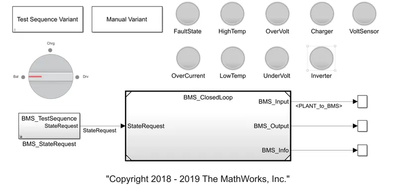
Test Case 1: -
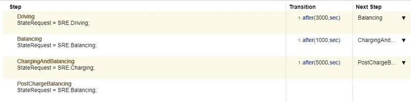
We can observe from this flow chart that driving is done for 3000 seconds and then balancing is done for 4000 seconds, during which time the vehicle is in standby mode. The next stage after balancing is charging, which takes 9000 seconds. After that, post-charge balancing is carried out till the simulation is completed.
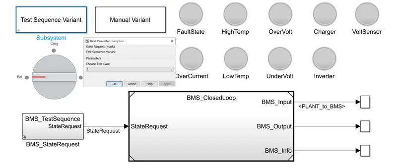
The Scope results for the first test in shown below:
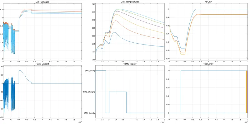
- The first plot shows us the individual cell voltages for 6 cells. The fluctuating voltage between 3.2 and 3.7 is provided during the driving state time (between 0 and 3000 seconds), indicating that the nominal voltage was 3.7 and it decreased to 3.2 per cell. During the charging phase, it rises to 4.2V. (Between 4000 to 9000 secs). The fully charged voltage of the battery is 4.2. Because the BMS was in standby mode, it did not diminish.
- The entire battery pack current is shown in the second plot. Because the battery loses current when driving, it is displayed in the negative direction (till -60A). The current rises to 30A during charging and then drop to zero during standby.
- The third figure depicts the battery pack's cell temperatures, which range from 290K to 315K. The temperature of the cells rises during battery depletion and gradually drops during charging and standby mode. We can observe from the graph that the sixth cell has the highest temperature, indicating that it is discharged the most.
- The BMS states are depicted in the fourth plot. As previously stated, the driving time ranged from 0 to 3000 seconds, the charging time ranged from 4000 to 9000 seconds, and the standby time ranged from 9000 to 20000 seconds.
- The fifth graph depicts the SOC in three separate graphs, with the SOC rapidly decreasing to 0.4 during driving and fully charging back to 100% during driving. In standby mode, the SOC will not change.
- The cell balancing signals are shown in the sixth block. From the sixth cell of the battery pack to the first cell, the balancing of cells is presented in descending sequence. The temperature block in the cell confirms this.
Test Condition 2:

The driving state is maintained until 10000 seconds have passed, following which charging begins.
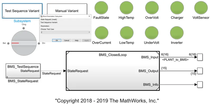
The scope results for the second test are shown below,
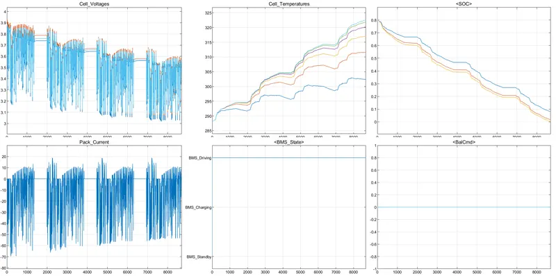
- The BMS enters driving mode in this second situation until the battery pack's SOC is depleted. The battery pack discharges current for 8692 seconds, as seen in the graph. We may deduce from this that the battery pack lasts 8692 seconds on a single charge. Here, there is no charging or standby mode. The electric vehicle continues to run until the battery pack is entirely depleted.
- The voltages range from 3.7 to 3 volts. This 3V is the individual cell's cutoff voltage. The battery pack can discharge up to 60A of electricity, which is its maximum capacity. The temperature of the cells continues to rise as a result of the constant discharge of current. The SOC continues to fall until it hits 0%. Because the battery pack has not been charged or stood by, cell balancing is not performed while charging. The cells have been discharged evenly until they are shut off, hence there is no cell balancing signal.
- Using this sort of case scenario will allow us to better grasp the battery's endurance and life duration.
Test Condition 3:
The flow chart for this test condition is as follows,

There is just one BMS state shown in this flow chart, which is charging. So, from 0 to 20000 seconds, only charging takes place.
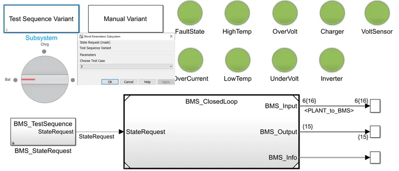
The scope results for the third test are shown below,
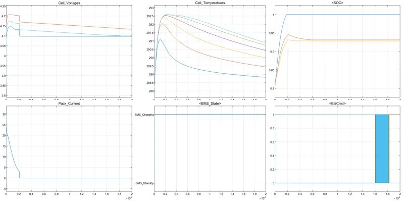
- The charging duration is fully in this third circumstance. There is no such thing as a driving or standby state. The SOC was set to 80 percent at first, and then the pack was fully charged. After being fully charged, the pack current increased to 30A and then decreased to zero. The in-rush current is limited by the contactor circuits. After being fully charged, the battery can no longer take current.
- The fully charged voltage range for the cell is between 4 and 4.2 volts. The cell temperatures were also somewhat higher at first due to the initial charging current, but they quickly stabilized thanks to the contactors. According to the plot, the balancing orders were followed from the sixth cell to the first cell.
- As a result, the BMS system was thoroughly examined, and the three separate test case situations were thoroughly discussed.
#2 What is coulomb counting? Refer to the above model and explain how BMS implements coulomb counting for SOC estimation?
Coulomb Counting Method:
The Coulomb counting method estimates SOC by measuring the discharge current of a battery and integrating it over time. The SOC(t), which is determined using the discharging current, I(t), and previously estimated SOC values, SOC, is calculated using the Coulomb counting technique (t-1). The following equation is used to determine SOC:
`SOC (t)= SOC(t-1)+{I_c(t)}/Q_n Deltat`
Flow Chart for Coulomb Counting:
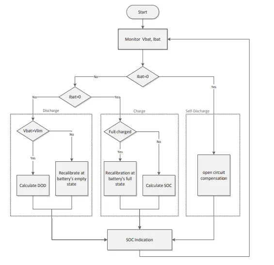
The SOC of a Li-Ion battery is estimated using this approach by monitoring both the voltage `V_{bat}` and the current `I_{bat}`. The direction of current via the battery system identifies the battery's operation mode.
When the battery is in open circuit mode, `I_{bat} = 0` and compensation of self-discharge losses will be taken into account as explained in sub-section C.
The battery voltage, current flowing through it, and operational temperature are all required for monitoring. Coulomb counter `Delta Q` is used to track the SOC when the battery is charged or discharged.
`Delta Q =int_t^{t+tau} I_{bat} dt` (2)
This variance `Delta Q` that will be used in the following equations is negative if the battery is in discharge, positive if in charge.
A. Charge Mode
In this mode, the coulomb counter is presented by ܳ`Q_{gained}` as expressed in (3), which represents the number of charges accumulated during `tau`
`Q_{gained}(t+tau) = Q_{gained}(t)+DeltaQ` (3)
So, the variation of the state of charge gained in this same operating period is obtained by the relation (4)
`DeltaSOC(t+tau) = {Q_{gained}(t+tau)}/Q_{rated}*100%` (4)
We may get the instantaneous value of SOC by adding the prior state of charge indicator and the acquired one.
`SOC(t+tau)=SOC(t)+DeltaSOC(t+tau)` (5)
Knowing the relationship indicated about (6) the value of depth of discharge DOD is updated in every charging operation to get it back every switching to discharging mode.
`SOC(t)+DOD(t) = 100%` (6)
B. Discharge Mode
In the discharging mode the coulomb counter is presented by `Q_{lost}`, which represents the amount of charges losses in the operating period `tau` by equation (7):
`Q_{lost}(t+tau) = Q_{lost}(t) + DeltaQ` (7)
The depth of discharge variation is derived using (8) and utilized in (9) to determine the DOD value.
`Delta DOD(t+tau) = {Q_{loss}(t+tau)}/Q_{rated}*100%` (8)
`DOD(t+tau) = DOD(t) + DeltaDOD(t+tau)` (9)
After that, the equation (6) is used to determine the SOC
C. Self-Discharge Mode
At the battery storage periods, the percentage of monthly self-discharge is converted to the amount discharged per hour; this amount is designed by the constant q(per/hour). Considering a 5% rate of self-discharge per month q(per/hour) is approximated to 0.0016 Ah. So, the quantity of charges dissipated in the open circuit period ܳ`Q_{oc}` is calculated by equation (10) representing the accumulative losses during the store hours.
`Q_{oc}(h+1) = Q_{oc}(h) +q_{per /hour}` (10)
ℎ: Hour of storage
This value will be added to the amount of charge lost ܳ`Q_{lost}` during discharge mode and subtracted from the amount of charge accumulated ܳ`Q_{gained}` in charge mode as expressed in relations (11) and (12). This compensation of self-discharging loss is made at each open circuit period and before switching to another operating battery’s mode.
`Q_{lost}=Q_{lost} + Q_{oc}` (11)
`Q_{tot}=Q_{tot} - Q_{oc}` (12)
D. Temperature effect
The temperature variation affects considerably the state of charge of the Li-Ion battery [16]. To improve the accuracy of the battery state of charge, a temperature coefficient ߙ is introduced and multiplied by the value of the calculated SOC [17]. This coefficient varies depending on the operating temperature according to the interval's variations (13)
`{(0.5, T<-20^o),(1, -20^o<=T<=40^o),(0.8, T>40^o):}` (13)
E. Recalibration
When the loaded voltage ܸ`V_{bat}` drops under a limit voltage `V_{lim}` (3V), during the discharging mode the battery is considered totally discharged. When it’s empty, the battery can no longer be used and should be recharged. So, after a cycle of charge/discharge, a recalibration should be made of `Q_{max}` which represents the maximum capacity that can be released by the battery. This recalibration allows rectifying the
indication of SOC by replacing ܳ`Q_{rated}` by `Q_max`in relation (4). Also, we recalibrate the State-of-Health (SOH) of the battery SOH defined is a relation (14) as:
`SOH(nc) = {Q_{max}(nc)}/{Q_{rated}}*100%` (14)
Refer to the above model and explain how BMS implements coulomb counting for SOC estimation?
To compute the estimated soc of the battery management system, we must insert the plant block into this model, which incorporates BMS ECU and PLANT.
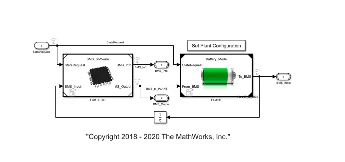
We require an accurate estimate of battery SOC before we charge our car. In the battery system, we don't assess the state of charge; instead, we measure things like battery pack current, cell voltage, and cell voltage using signals from the plant.
after entering the plant block, we can see the state machine, SOC estimation, and balancing logic block.
In this section, we'll look into SOC estimate.
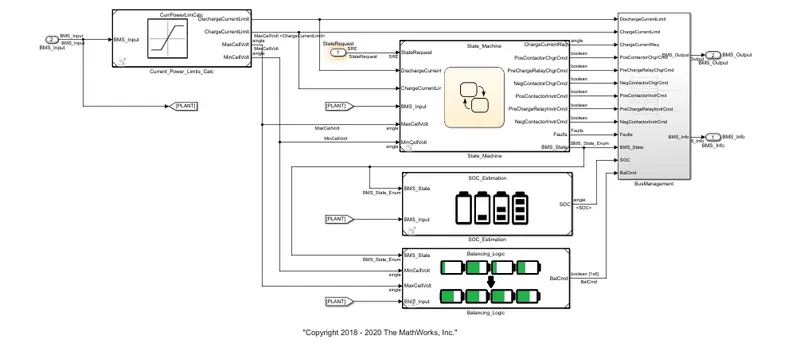
Three distinct state of charge estimating strategies are shown in this SOC estimate block. Each strategy has its own set of benefits and drawbacks. Columb counting is the first approach, while unscented(ukf) and extended Kalman filter are the other two (ekf). We're talking about the Columb counting approach here.
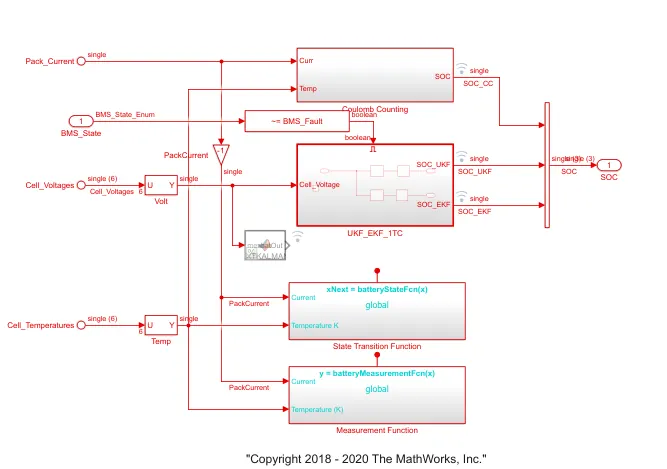
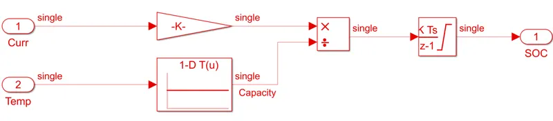
In coulomb counting method block
It accepts two input signals: current and temperature, with the current signal going to the gain block and the temperature signal going to the battery time and current lookup tables. Both blocks are linked to the split block, and these signals are sent to the discrete-time integrator to track the charge, which then aids in the calculation of the state of charge.
The positives of this are its simplicity and cheap capital cost, while the disadvantages include a buildup of current sensor error and its inability to recover from the erroneous start condition. due to a lack of voltage measurement feedback
Conclusion:
1)One of the most difficult aspects of coulomb counting is calibrating the initial battery SOC. In various applications, rest is required for startup, and the initial SOC is calculated using the voltage.
2)Kalman filtering is a technique for estimating unknown variables based on observations collected over time.
References: