Week 7 State of charge estimation
1. Simulate the 3 test cases from the harness dashboard and write a detailed report on the results
We download the project model from the Matlab link that was provided and simulate it for different drive cycles.
1. We select the first option from the test sequence variant and simulate it. The harness dashboard output after the simulation is given below.
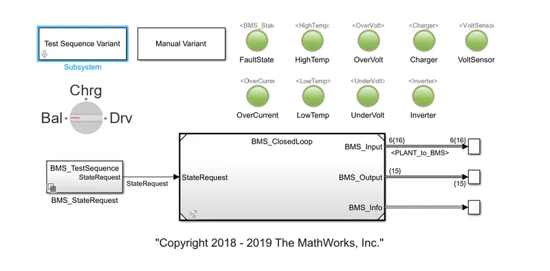
The green indicates the particular parameters are working on a set of the desired range of safe operating conditions. The plots of all the indicators are shown below we can cross-check this with the input provided.
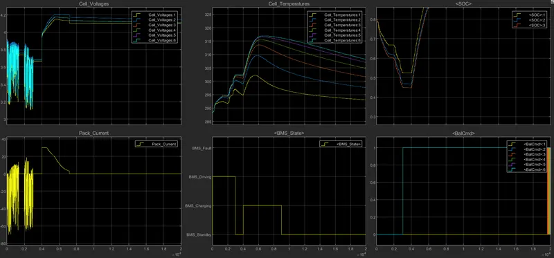
As per the input, the vehicle is in driving mode for 3000 sec, goes on standby for 1000 sec, and charges for 5000 sec and standby for the rest of the simulation. The same change in plot character can be visible in all the plots. As the vehicle moves voltage fluctuates between 3.2 to 3.8. By charging constant current the voltage raises to 4.2 for 1000 sec and undergoes constant voltage and the current which was at 30 drops back to 0 over time. While driving mode, the temperature gradually raises, and by charging the temperature increases further high. The SOC also fluctuates over time to 0.5 over driving mode and back to 100 by charging.
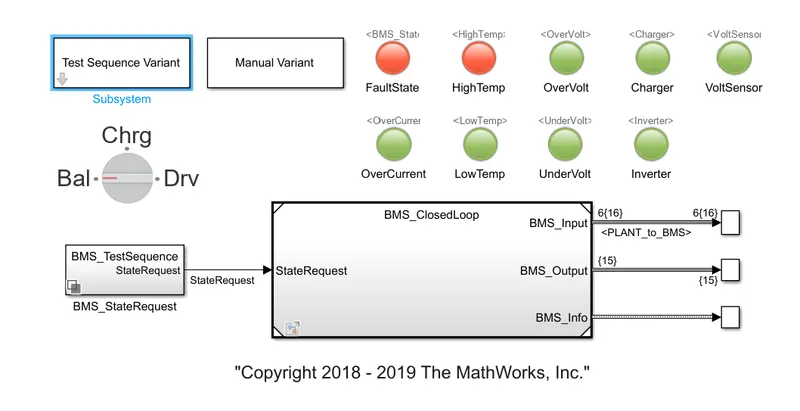
2. Now we select the 2nd option and proceed with the simulation and we get the result below that fault state and high temperature.
We consider the graphical plot in order to understand more about the fault indicated.
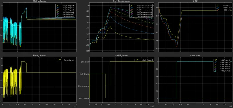
The system undergoes drive mode for 5000 sec and switches to charging mode. We can find that one of the cell temperatures reaches a maximum operating temperature of 320 to 325 range and the Fault state and high temperature get alerts, followed by which all other operations get terminated and the indicators come to a steady and normal state.
3. We select the 3rd option and run the simulation.
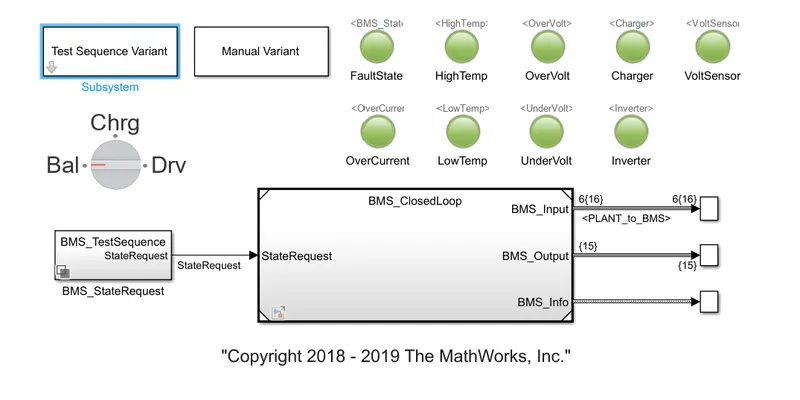
The indicators are green and we have successfully simulated the state request input. Now the indicator plots are given below.
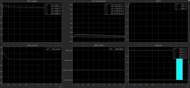
This is a pure charging cycle as per the BMS state plot. The SOC increases from 80 to 100 over time and stays in full charge over the period. Voltage stays constant until SOC becomes 100 % and current decreases to 0. Since there is no remarkable work done, the temperature slightly varies and kept its constant range.
2. What is coulomb counting? Refer to the above model and explain how BMS implements coulomb counting for SOC estimation.
The SoC of a battery cell is required to maintain its safe operation and lifetime during charge, discharge, and storage. However, SoC cannot be measured directly and is estimated from other measurements and known parameters. This leads to errors in the estimated SoC and that means it is not possible to fully exploit the full capability of the cell.
Coulomb counting gives a relative change in SoC and not an absolute SoC. If you measure the current over a given time step you have a measure of the number of Ah that have left or been received by the battery.
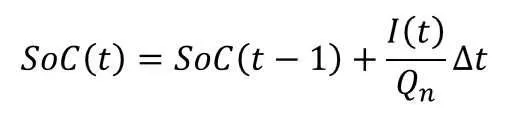
where:
- SoC(t) = estimated the State of Charge at the time, t
- SoC(t-1) = previous State of Charge at time t-1
- I(t) = charging or discharging current at the time, t
- Qn = battery cell capacity
- Δt = time step between t-1 and t
We look into the BMS ECU diagram given below to know the SOC estimation model.
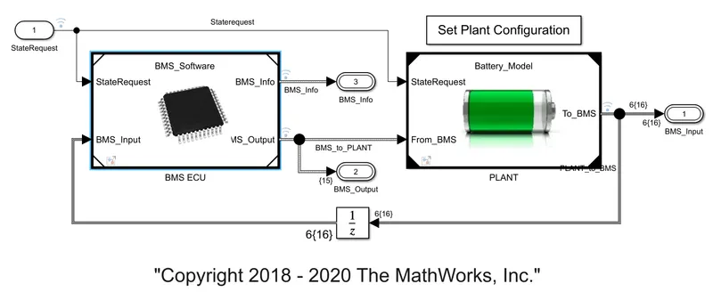
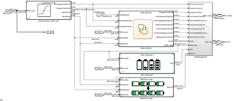
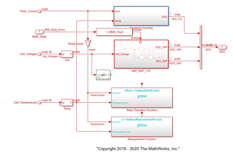
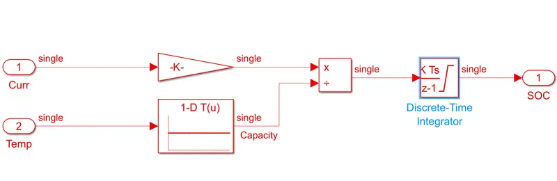
From the BMS subsystem, we can find the above subsystems to get to the last screenshot where we give current and temperature as input and undergo the above-mentioned calculation to give the SOC estimation.