Project 1

PROJECT NAME

The development of a forward energy-based fuel consumption model of a conventional vehicle.

PROJECT AIM

• Build Simulink model using blocks and complete the vehicle Model
• Write scripts in MATLAB to load all the variables needed to run the simulation model.
• Analyse data and create plots using MATLAB scripts.

PROJECT OBJECTIVE

1. Tabulate the fuel economy numbers (kmpl) for UDDS and HWFET cycle. This forms the baseline numbers for comparing with the future hybrid version.
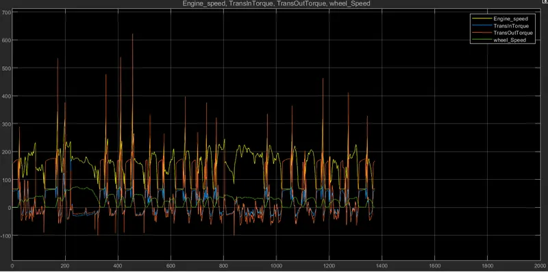
2. Plot the time trace for engine, transmission input, transmission output and wheel speed on one plot.
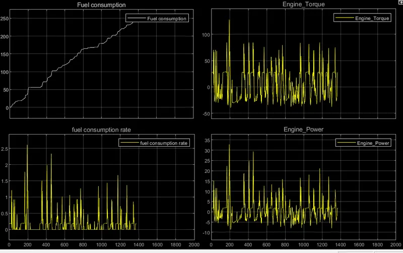
3. Plot engine torque, engine power, fuel rate and fuel consumption using subplots.
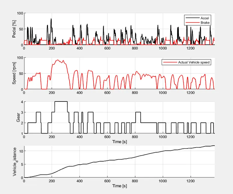
4. Plot accelerator and brake pedal, gear command, vehicle desired and actual speed, vehicle distance using subplots.
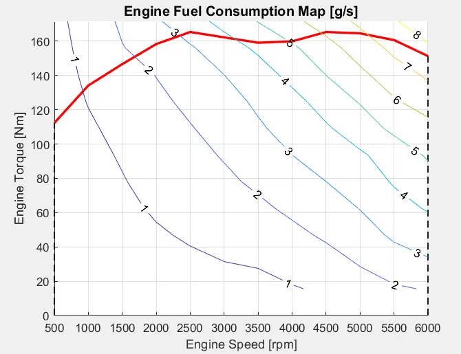
5. Plot the engine operating points on the engine fuel map.
6. Write down appropriate brief comments on each of these plots, describing the vehicle behavior throughout the drive cycle.
7. Generate the plots for both drive cycles.

INTRODUCTION

• In the forward scheme, a driver model controls the vehicle in an attempt to follow the input driving cycle, and the vehicle speed is intrinsically a dynamic state.
• A driver controller is required to control the vehicle to follow a desired speed and set the start of the calculations. The controller is implemented to model the driver that will either push the accelerator or the brake pedal to match the desired speed which enables to study the driver behaviour. The controller is used as part of a feedback loop that will determine the energy required to drive the vehicle.
• Analytical models are representative of the Vehicle behaviour and can be developed in MATLAB/Simulink by creating an vehicle model. They are based on fundamental theoretical equations. A model of the vehicle dynamics is built based on vehicle dynamics theory to calculate the power required at the wheels to overcome the resistances forces opposed to the vehicle motion: Aerodynamic Drag, Rolling, Inertia, Gradient and Transmission resistances. The power required derives from the tractive force expressed as the sum of the resistances forces above
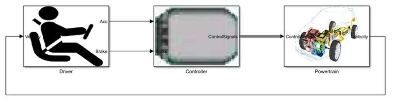
• The Simulink model for the convection model is created using 3 main subblocks for the driver model, control model and powertrain block.
• The actual vehicle speed is given as feedback to the driver block, and the driver block gives the controller block the required acceleration or brake output, while the controller block provides control signals for engine torque, gear shifting and brake torque to the Powertrain model.

VEHICLE PARAMETRS

• Using Matlab script ,the vehicle parameters are introduced to the vehicle simulation for running the model and plotting the required outputs.Drive cycle selection is also done from here. Before running the Simulink vehicle model, the script is initialized at MATLAB to load all the variables in the workspace.

%%%%%%%%%%%%%%%%%%%%%%%%%%%%%%%%%%%%%%%%%%%%%%%%%%%%%%%%%%%%%%%%%%%%%

%% Skill-Lync -> Hybrid Drives Development

% Project 1 - Conventional Vehicle Model

% By - ARJUNDEV V V

% Description:

%% Initialization File

% Initialization file for loading the variables for the Conventional vehicle simulation model

%% Vehicle Parameters

M = 1500; % Vehicle weight [kg]

Cr = 0.015; % Rolling resistance coefficient

Rw = 0.35; % Rolling radius [m]

Cd = 0.33; % Drag coefficient

Af = 2; % Frontal area [m2]

rhoa = 1.225; % Air density [kg/m3]

Vwind = 0; % Wind velocity [kmph]

g = 9.81; % Gravitational acceleration [m/s2]

theta = 0; % Slope [deg]

myu_road_tire = 1; % Coefficient of friction between tire - road interface

%% Powertrain Parameters

FDR = 3.73; % Final Drive Ratio / Diff Ratio

DiffEff = 0.99; % Differential efficiency (assumed independent of operating conditions)

NumGear = 4; % Number of gears in transmission

TransGear = 1:NumGear; % Transmission Gears

TransRatio = [3.06, 1.62, 1, 0.7]; % Corresponding Transmission ratios

TransEff = 0.90; % Transmission efficiency (assumed independent of operating conditions)

TC_SR = [0, .5, .6, .7, .8, .87, .92, .94, .96, .97, 1]; % Torque Converter Speed Ratio (Matlab default) -> TurbSpd/PumpSpd

TC_TR = [2.232, 1.5462, 1.4058, 1.2746, 1.1528, 1.0732, 1.0192, 1, 1, 1, 1]; % Torque Converter Torque Ratio (Matlab default) -> TurbTrq/PumpTrq

TC_Cf = 1e-4 * [.72558, .66322, .63463, .59042, .51331, .4144, .29287, .22444, .12186, .04386, 0]; % Torque Converter Capacity Factor (Matlab default) -> PumpTrq/PumpSpd^2 [Nm/rpm^2]

load Vehicle_Data/Engine_data_1_9L_Saturn_95kW

load Vehicle_Data/Trans_Shift_map

%% Driver Parameters

Kp = 10; % P gain for driver PI model

Ki = 1; % I gain for driver PI model

Drive_Cycle_Select = 1; % Drive cycle selection

% Drive cycle values in m/s

if Drive_Cycle_Select == 1

load DriveCycles/UDDS;

elseif Drive_Cycle_Select == 2

load DriveCycles/HWFET;

elseif Drive_Cycle_Select == 3

load DriveCycles/FTP;

elseif Drive_Cycle_Select == 4

load DriveCycles/US06;

elseif Drive_Cycle_Select == 5

load DriveCycles/NEDC;

elseif Drive_Cycle_Select == 6

load DriveCycles/WLTP;

end

time_end = cyc_time(end);

vel_end = cyc_vel(end);

VEHICLE DESIGN (SIMULINK)

• The Simulink is used to create the basic model for our conventional vehicle using 3 main subsystems Driver model , Controller model , powertrain model

Driver model:

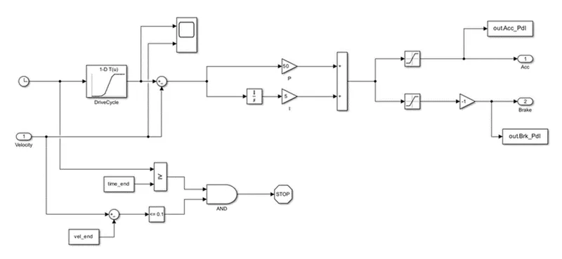
Driver Model is a basic PI controller that generates accelerator and brake pedal outputs to match the desired and actual vehicle speed . The schematic diagram for the driver model is shown below.

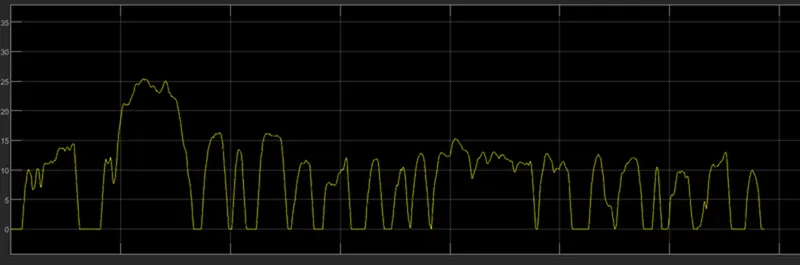
The scope graph created for input drver velocity signal.

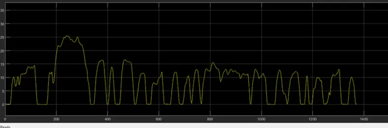
The feedback velocity signal is shown below.

Controller model :

Based on the driver inputs the controller generates desired engine torque, desired transmission gear and desired brake torque. These inputs are fed to the ‘Powertrain’ block which represents the drivetrain of the vehicle.The PI controller controls the error between the required drive cycle and actual vehicle speed by providing acceleration and brake pedal output to the controller.

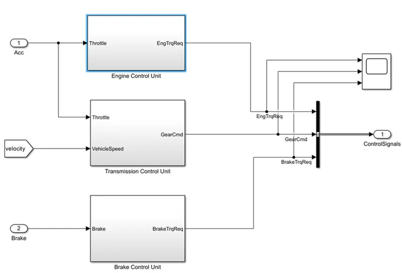
The controller consists of an engine control unit, a transmission control unit and a brake control unit.

The graphical scope output of engine torque , gear command , breake torque required.

Engine Control Unit:

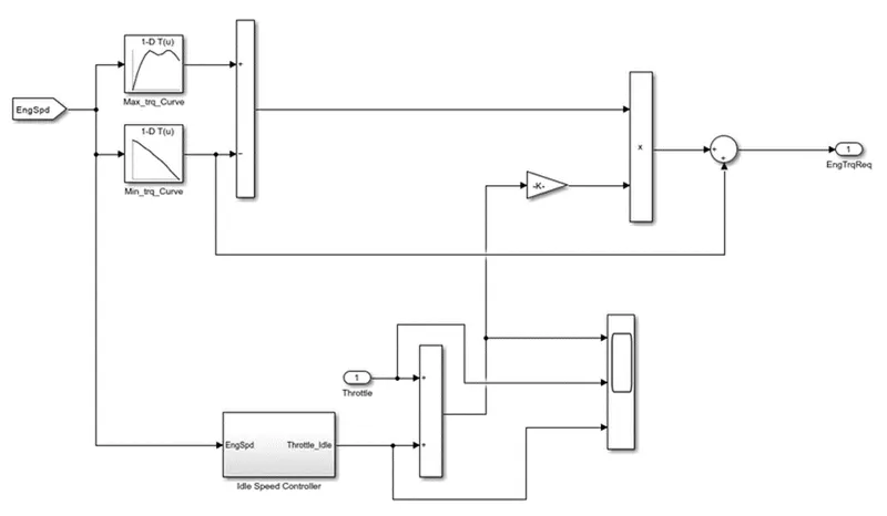
Graph created from the scope is given below.

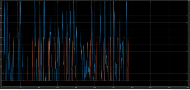
Idle Speed Controller:

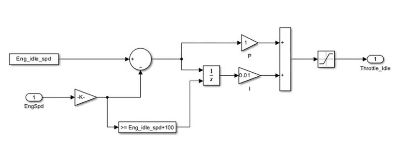
Transmission Control Block :

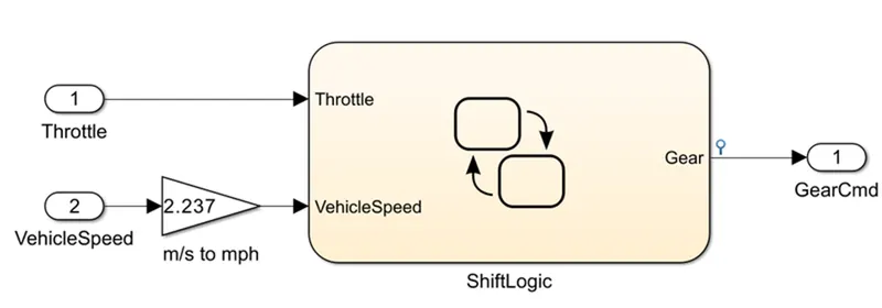
The transmission control block controls the gear shifting using the study flow Variable chart.

Brake Control Unit :

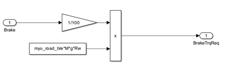
Brake Control unit Produce required brake torque according to the brake pedal input and passes the brake torque in to the wheel block in the transmission model.

Powertrain model :

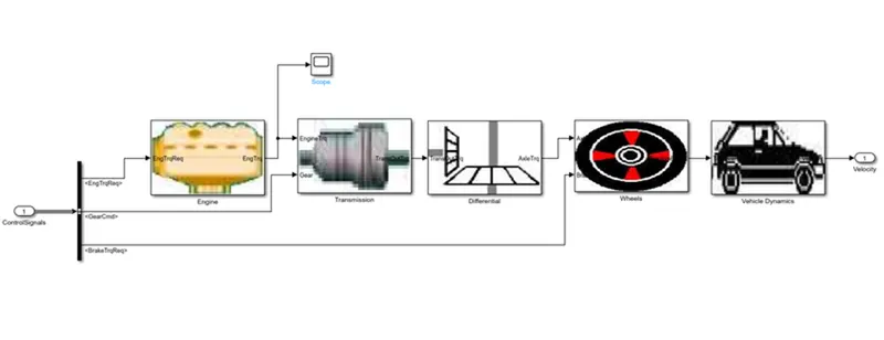
The powertrain model includes all the components that convert the power of the engine into vehicle motion. It has 5 subsystems that are Engine , Transmission , Differential , Wheels , vehicle Dynamics.

Engine Model:

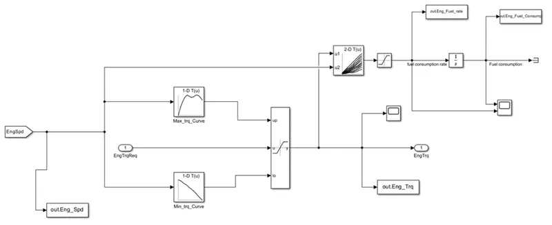
• Based on the Engine speed The required torque from the controller is saturated between Max torque curve and min torque curve and passes the Engine torque to the Transmission block
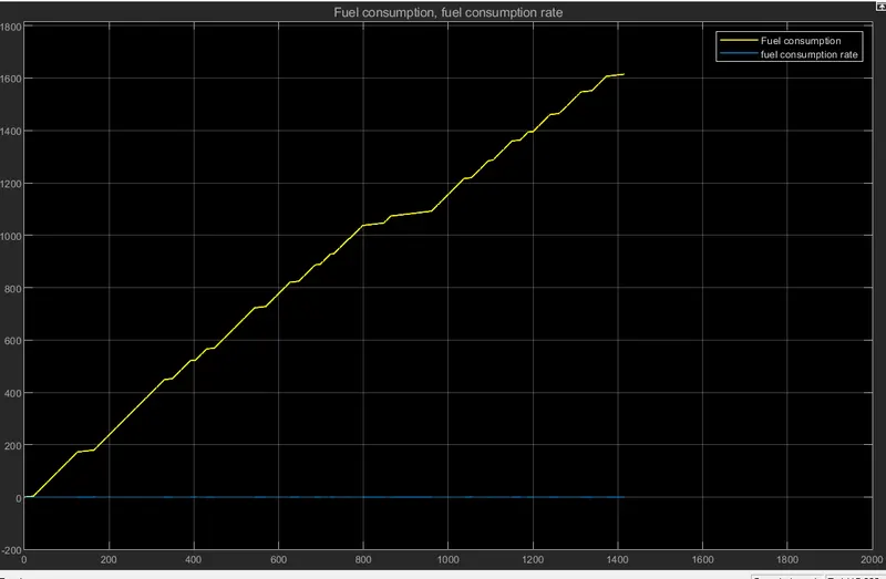
• The 2D lookup table is used to calculate the fuel flow rate based on engine speed and engine torque. The fuel flow rate is then integrated to find the fuel consumption.
• Estimated fuel flow rate, fuel consumption, engine torque and engine speed are passed to the MATLAB workspace using the to-workspace block.

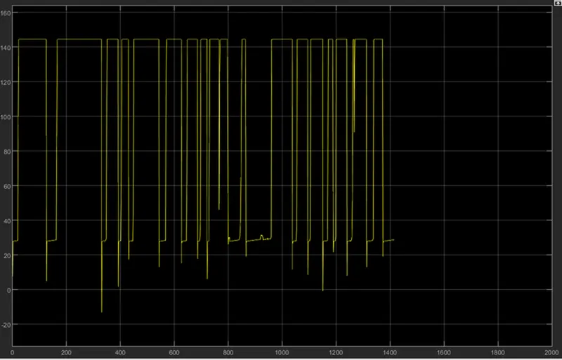
The graph created from scope of Engine torque output .

The transmission unit :

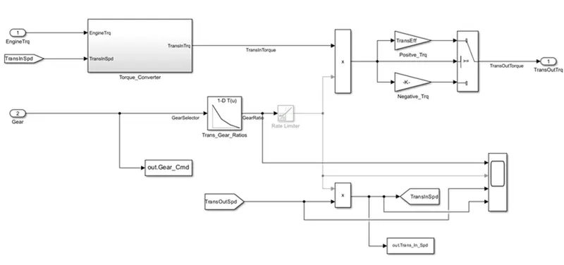
In these model we take engine torque, gear selector from controllerb for transmission of gear ratio. The ratio is multiply by transmission input torque and then the transmission efficiency positive torque and negative torque gives transmission input speed. In this case torque converter connects the engine to transmission it is part of transmission. In it basically engine dynamics and that is decoupled.

Differential :

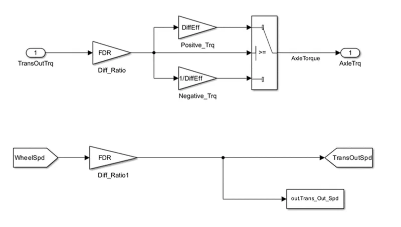
In this taking input is the transmission output then its going to the differential ratio multiplied the output and input torque then meet axle torque. The axle torque is a lower than the transmission torque and differential ratio.

Wheels:

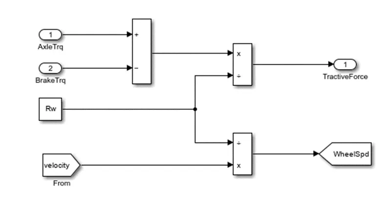
In this model we take the axle torque from differential and brake torque from controller. it is subtracting and multiplied rolling radius and velocity then we meet the tractive force from axle and brake torque. and the wheel speed is meet using velocity.

Vehicle Dynamics:

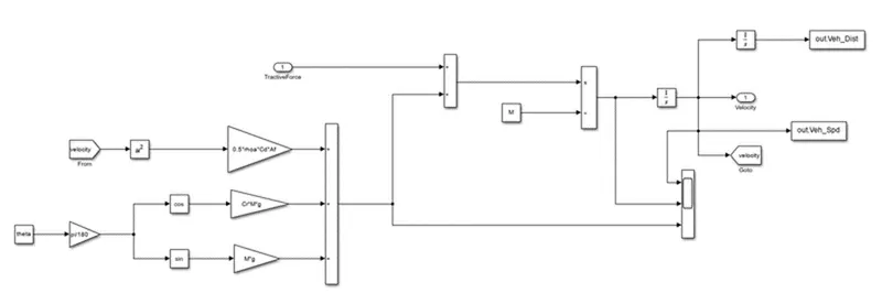
In this takes tractive force and road load. It is dictates vehicle speed based on tractive force and road load.

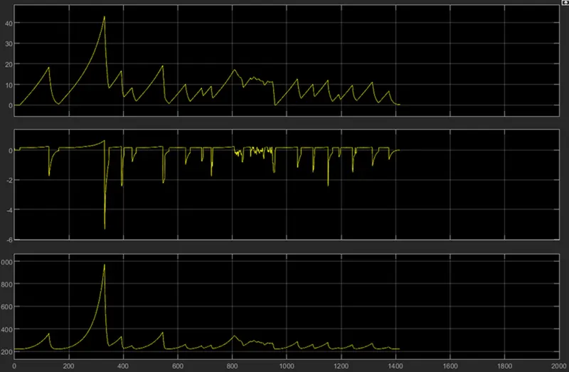
Graph created from Scope in Driver Model: - Road load , Acceleration , vehicle velocity

the dynamic equation for calculating road load is

where,

p = air density [kg/m^3]

A = Frontal area [m^2]

Cd = drag Coefficient

Vveh = velocity of vehicle [m/s^2]

Vwind = velocity of wind [m/s^2]

Cr = rolling resistance coefficient

M = mass in [Kg]

g = gravity.

Then we calculate and integrate then we meet acceleration of vehicle and velocity of vehicle it means vehicle distance and vehicle speed.

Post processing of the model

%%%%%%%%%%%%%%%%%%%%%%%%%%%%%%%%%%%%%%%%%%%%%%%%%%%%%%%%%%%%%%%%%%%%%

%% Skill-Lync -> Hybrid Drives Development

% Project 1 - Conventional Vehicle Model

% By - ARJUNDEV V V

% Description:

% The following file is to used with the Initialization file and Simulink

% results for post-processing of the data.

% The file is incomplete, has some examples of how the data is imported

% into a readable format, data analysis and plotting examples.

% Based on the project task, use commands in a similar format as given

% below, to analyse the data and generate required plots.

% You can change variable names if desired

%% Post-Processing File

% File for post-processing the Conventional vehicle simulation model data

%% Renaming variables

Time = out.tout;

Acc_Pdl = out.Acc_Pdl; % Accelerator pedal [%]

Brk_Pdl = out.Brk_Pdl; % Brake pedal [%]

Gear_Cmd = out.Gear_Cmd; % Transmission gear

Trans_In_Spd = out.Trans_In_Spd*30/pi; % Transmission input speed [rpm]

Trans_Out_Spd = out.Trans_Out_Spd*30/pi;% Transmission output speed [rpm]

Eng_Trq = out.Eng_Trq; % Engine brake torque [Nm]

Eng_Spd = out.Eng_Spd*30/pi; % Engine speed [rpm]

Eng_Fuel_Consump = out.Eng_Fuel_Consump; % Engine fuel consumption [g]

Veh_Dist = out.Veh_Dist/1000; % Distance traveled by vehicle [km]

Veh_Spd = out.Veh_Spd*18/5; % Vehicle speed [kmph]

%% Data Analysis

Eng_Pwr = Eng_Spd*pi/30*Eng_Trq/1000; % Engine brake power [kW]

rho_petrol = 0.7197; % Density of petrol [kg/L]

kmpl = Veh_Dist(end)/(Eng_Fuel_Consump(end)/1000/rho_petrol); % Fuel economy [kmpl]

%% Plotting vehicle characteristics time trace

figure(1)

subplot(3,1,1)

hold on

grid on

plot(Time, Acc_Pdl, 'linewidth', 1, 'Color', 'black');

plot(Time, Brk_Pdl, 'linewidth', 1, 'Color', 'red');

ylabel('Pedal [%]')

xlim([0, Time(end)]);

legend('Accel','Brake');

subplot(3,1,2)

hold on

grid on

plot(Time, Trans_In_Spd, 'linewidth', 1, 'Color', 'black');

plot(Time, Trans_Out_Spd, 'linewidth', 1, 'Color', 'red');

ylabel('Speed [rpm]')

xlim([0, Time(end)]);

ylim([0, 6000]);

legend('Trans Input','Trans Output');

subplot(3,1,3)

hold on

grid on

plot(Time, Gear_Cmd, 'linewidth', 1, 'Color', 'black');

xlim([0, Time(end)]);

xlabel('Time [s]');

ylabel('Gear');

%% Plotting engine operating points on engine fuel map

figure('Name','Engine Operating Points');

hold on

grid on

title('Engine Operating Points','fontsize',12);

p1=plot(Eng_map_spd*30/pi,Eng_max_trq,'linewidth',2,'color','r');

p2=line([Eng_map_spd(end)*30/pi Eng_map_spd(end)*30/pi],[0 Eng_max_trq(end)]);

set(p2,'linewidth',1,'linestyle','--','color','k');

p3=line([Eng_map_spd(1)*30/pi Eng_map_spd(1)*30/pi],[0 Eng_max_trq(1)]);

set(p3,'linewidth',1,'linestyle','--','color','k');

[c,h] = contour(Eng_map_spd'*30/pi,Eng_map_trq,Eng_fuel_map');

clabel(c,h);

xlabel('Engine Speed [rpm]');

ylabel('Engine Torque [Nm]');

title('Engine Fuel Consumption Map [g/s]');

p4 = plot(Eng_Spd,Eng_Trq,'--','color','k');

legend([p1 p4],{'Max Curve','Operating Points'});

axis([Eng_map_spd(1)*30/pi Eng_map_spd(end)*30/pi 0 Eng_map_trq(end)]);

PLOTS AND STUDY

UDDS :

1, Drive cycle-

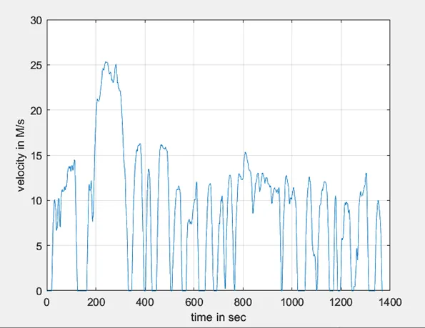
1.Tabulate the fuel economy numbers for UDDS cycle.

2. Plotting Vehicle characteristics time trace for engine, transmission input, transmission output and wheel speed

3.Plotting Engine torque,engine power, fuel rate and fuel consumption using subplots

4. Plotting accelerator and brake pedal, gear command, vehicle desired and actual speed, vehicle distance using subplots

5. Plot the engine operating points on the engine fuel map.

HWFET:

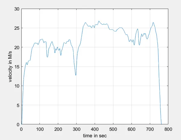
1.Tabulate the fuel economy numbers for HWFET cycle.

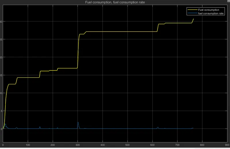
As per the required velocity demand in the HWFET cycle the fuel consumption increases drastically compared to the UDDS cycle where the fuel consumtion is linear due to velodity demand there.

2. Plotting Vehicle characteristics time trace for engine, transmission input, transmission output and wheel speed

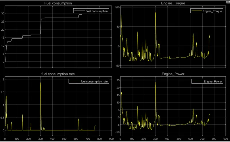
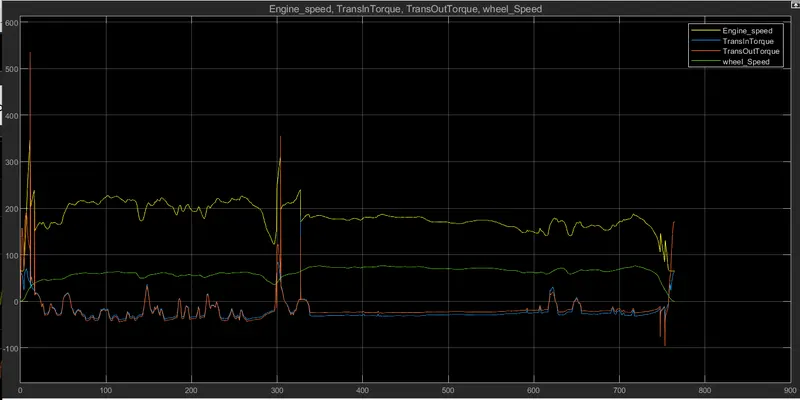The torque requirements of the drive cycle are different and the fuel flow rate varies and fuel consumption is calculated.The HWFET drive cycle has higher power and torque requirements and less negative torque and power compared to UDDS.

3.Plotting Engine torque,engine power, fuel rate and fuel consumption using subplots

4. Plotting accelerator and brake pedal, gear command, vehicle desired and actual speed, vehicle distance using subplots

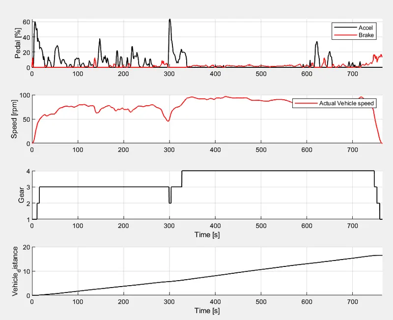
From the above the study we can see that the axle pedal and break pedal are not used freaquently as compared to UDDS demand where freaquent axle and brake pedals are applied . AS per that the velocity remains in an mean position for highway demand and the gears are not shifted freaquently.

5. Plot the engine operating points on the engine fuel map.

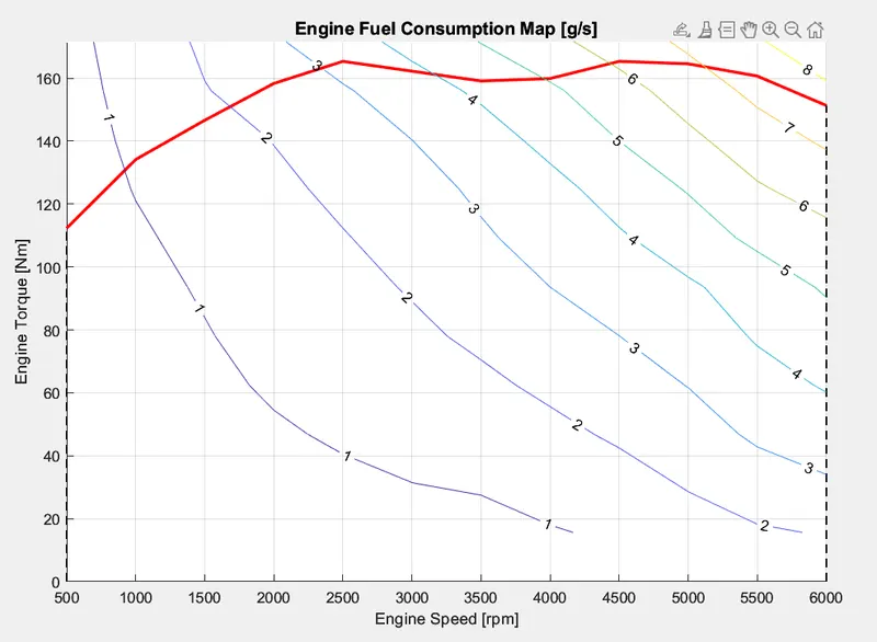The engine operating points are plotted on the fuel map and the operating point is under the maximum torque curve.

CONCLUSION

• The development of a forward energy-based fuel consumption mol of a conventional vehicle is developed using Matlab and simulink .
• Analysis and understands vehicle operating points based on engine speed, torque, transmission speed, axle and brake pedal positions, gear, and distance travelled.
• The fuel consumption and fuel consumption rate for each drive cycles are compared.
• Post process calculations were performed and the required graphs were successfully plotted.