Week 7 State of charge estimation

Battery Management System:

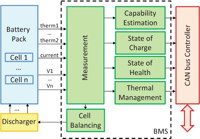
The below flow chart gives the Implementation of BMS for a Battery Pack comment Share Project The below flow chart gives the information of BMS working in coordination with the battery pack. The inputs to the BMS from the battery pack will be mainly the Current, Voltage and Temperatures. And based on the inputs obtained from the battery pack the BMS will be giving the outputs as SOC, SOH, Thermal Management and Capability of total battery pack. All the BMS outputs are given to CAN bus controller to communicate with the Dash board of the vehicle or to the user and also with the charger and others. Here cell balancing is also implemented to make sure the maximum battery pack is fully utilized to its full charging and discharging capacity.

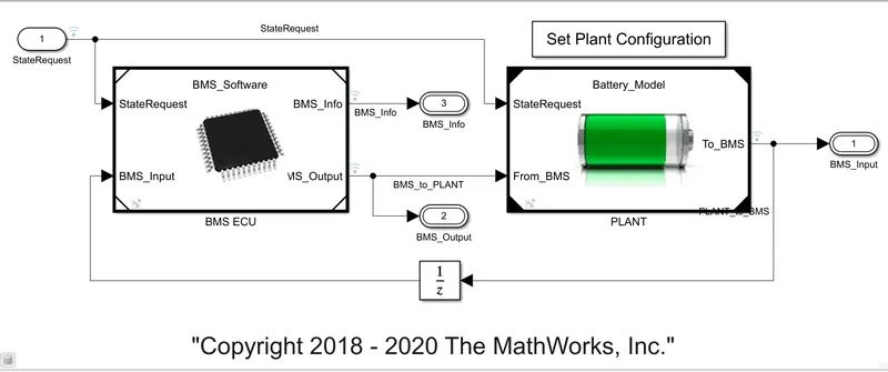
This is how the BMS is implemented in the MATLAB along with the battery pack.

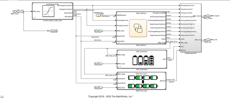
This is how BMS is modelled inside from the subsystem of BMS ECU

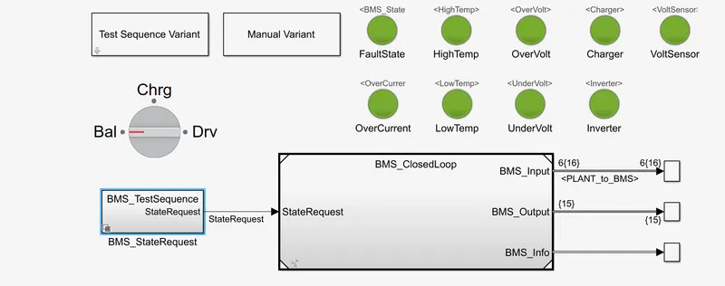
From the above MATLAB model, we are Simulating 3 test cases from harness dashboard to find out the fault condition in BMS. And the below image shows the dash board where we can get the information related to the faults like over voltage, under voltage, high temperature, over current and inverter related faults. If there is any fault condition the indicators will turn to red colour otherwise it shows the green indication means there is no fault and the system is safe. we can also know the information like the battery pack is in which condition at present moment like the mode of operation called Balancing mode, Charging mode and Discharging mode.

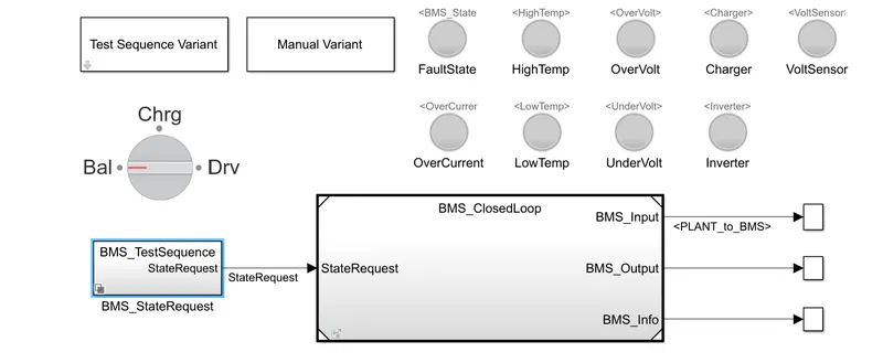
From the Test Sequence Variant we can implement the three Test conditions.

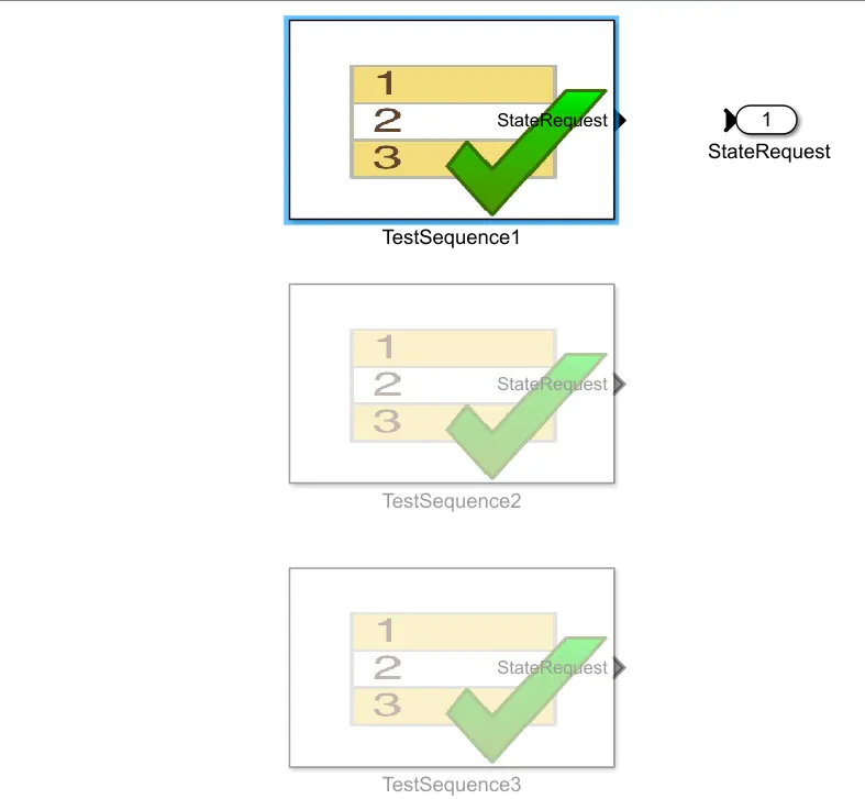
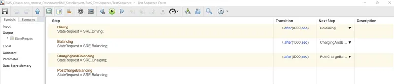
Test case 1: Discharging, Charging and Balancing / At BMS Level Test Condition For Both Driving & Charging.

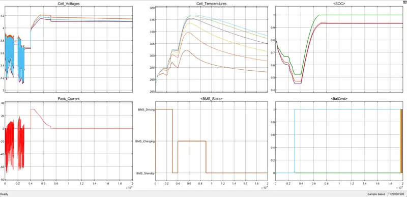
From the results of Cell Voltages and Pack Current:

We can observe the constant current (CC) and constant voltage (CV) characteristics of a battery pack. Initially the cell voltage is around 3.8V and the cell current is zero when the battery is fully discharged.

At time instant of 4000 sec the cell voltage is gradually increased from 3.8 to 4.2V at this same instant of time the peak current of cell increased from 0 to 30A and it is constant till 4525 sec this phase of cell is called a CC Mode and then it gradually reduces to zero at 7211 sec

At time 5516 sec the cell voltages are increased to 4.2V and then became constant from 7000 sec till the end of simulation time or till is completely charged this phase is called constant voltage CV Mode. usually, the CV mode takes longer time period than the CC mode.

Generally, cell manufacturers design the CC Mode till the cell reaches 80% of its full capacity and from there the remaining 20% will be considered as CV Mode.

Output Results Comparison of BMS State condition with Cell Voltages, Pack Current, Cell Temperatures, SOC and Cell Balancing

1)Discharging Mode / BMS Driving:

At time instant 0 to 3000 sec Cell voltages reduced from 4.2V to 3.7V

Pack current reduced to 0

SOC is initially is of 80% and reduced to 45%

Cell temperatures increased from initial 288 to 301.7k and difference in increase is 13 k Cell Balancing is idle in this time period.

2)Charging Mode / BMS Charging:

At time instant 3000 to 9000 sec Cell voltages are constant from 4.2V this is called CV Mode Pack current increased from 0 to 30A and reached its full capacity and then after reduces to zero in this CV Mode.

SOC is initially is of 30% at this stage and increased to 100% or 1 to its full capacity.

Cell temperatures increased from initial 302 to 316 k and difference in increase is 14 k and gradually reduced because the cells are fully charged.

Cell Balancing is operating in this time period to ensure the maximum capacity reached by all the cells while charging in equal mode of operation.

Result of SOC:

As we can observe the SOC is estimated using different methods like

1)Coulomb counting: From the result the green graph showing this method where the SOC reached to 100% at time 6802 sec

2)UKF Kalman Filter: SOC Estimation from this method is 93%

3)EKF Kalman Filter: SOC Estimation from this method is 93% Both the Kalman Filter methods are overlapping each other and giving the output result of SOC Estimation same as 93%.

Test case 2: Discharging and No Balancing / At BMS Level Test Condition for Driving.

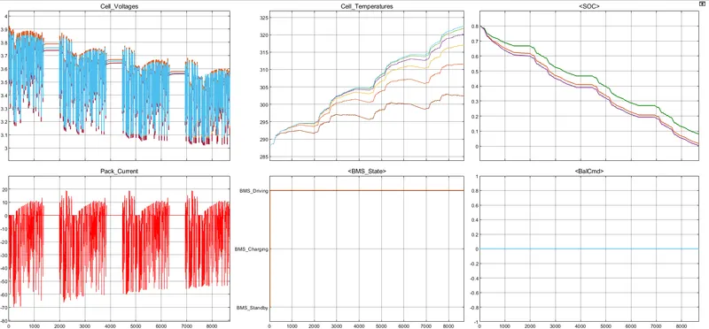
Output Results Comparison of BMS State condition with Cell Voltages, Pack Current, Cell Temperatures, SOC and Cell Balancing

1)Discharging Mode / BMS Driving: At time instant 0 till the end of simulation Cell voltages reduced from initial 4 V

Pack current reduced to 0

SOC is initially is of 80% and reduced to 0%

Cell temperatures increased from initial 288.15 k to a maximum recorded as 323 k and difference in increase is 34 k this increase is different and comparatively less with the maximum recorded as 323 k for other output graphs.

Cell Balancing is idle in this time period.

Hence there is no fault observed from the dash board where all the indication is green.

Test case 3: Charging and Balancing / At BMS Level Test Condition for Charging

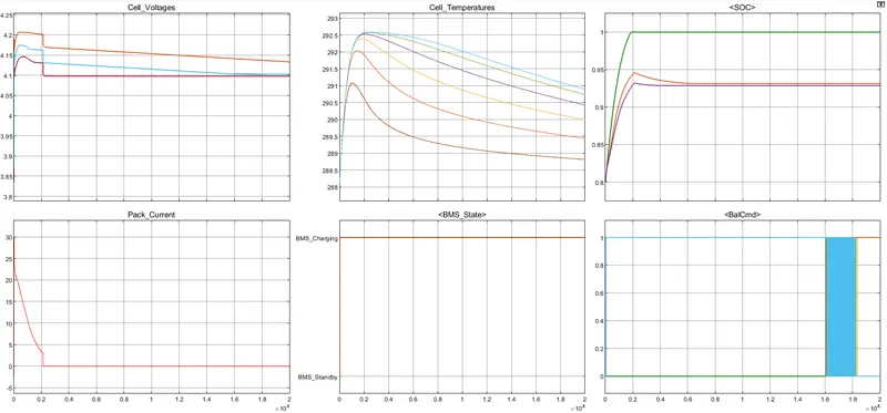
Output Results Comparison of BMS State condition with Cell Voltages, Pack Current, Cell Temperatures, SOC and Cell Balancing

1)Charging Mode / BMS Charging: At time instant 0 to till the end of simulation

Cell Voltages and Pack Current: we can observe the constant current (CC) and constant voltage (CV) characteristics of a battery pack.

From time period of 0 sec the cell current increased to 30A and the cell voltages also gradually reached to 4.2V this phase of operation is called constant current or CC Mode.

At time instant of 2000 sec the cell voltages are dropped and become constant till the end of the full charging voltage capacity of battery pack and at this time instant the current is gradually reduced to 0.

So, this mode of operation is called Constant voltage or CV Mode of operation. Generally, cell manufacturers design the CC Mode till the cell reaches 80% of its full capacity and from there the remaining 20% will be considered as CV Mode.

SOC (%) SOC is initially is of 80% at time instant of 1849 sec this is increased to 100% or 1 to its full capacity with variation in different SOC Estimation methods.

As we can observe the SOC is estimated using different methods like

1. Coulomb counting: From the result the green graph showing this method where the SOC reached to 100% at time 1849 sec
2. UKF Kalman Filter: SOC Estimation from this method is 93%
3. EKF Kalman Filter: SOC Estimation from this method is 93% Both the Kalman Filter methods are overlapping each other and giving the output result of SOC Estimation same as 93%.

Cell Temperatures: Cell temperatures increased from initial 288.1 k to a maximum recorded as 292.5 k with difference in temperature rise is 4.5 k recorded with other cell temperature estimation graphs.

Cell Balancing is operating in this time period to ensure the maximum capacity reached by all the cells while charging in equal mode of operation and at time period of 18000 sec the cell balancing is cut off.

SOC

SOC stands for the State Of Charge of a battery. SOC represents the amount of energy left inside the battery with respect to the total amount of energy in a battery at the Fully charged condition. SOC can help a user to determine when to charge the battery or stop charging and how much energy he can extract from a battery at that time. There is no direct method to calculate SOC for a Li-ion battery but there are several ways in which we can calculate SOC with the help of some additional parameters.

The easiest method to calculate the SOC of a battery is by using a battery voltage translation method. This method is not accurate but helps to approximately and quickly calculate SOC and can be used in devices like power banks where SOC is shown in range and not the exact percentage. For example, a typical power bank shows SOC in the range from 0-25%, 25-50%, 50-75%, 75-100%.

There are several limitations to this method and hence more accurate methods are needed like the Coulomb counting method, the Fuzzy logic method, the Kalman filter, the RBF Neural network, the Fuzzy neural network, the Hybrid methods, etc.

Each method has its limitations, accuracy, and complexity and hence proper decision should be made while selecting methods for SOC estimation.

Coulomb Counting Method:

The coulomb counting method is also known as the battery current integration method. In this method, a discharging/charging current I(t) is measured and integrated over time to calculate the amount of energy remaining inside the battery. In this method, SOC is taken at the previous time step SOC(t-1) and the amount of energy removed/added at the current time step is subtracted/added from the SOC of the previous time step SOC(t-1) to obtain the amount of energy present in the battery at the present instant.

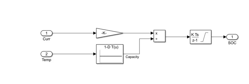
The SOC estimation in the coulomb counting method is done using the below equation,

`SOC(t) = SOC (t-1) * int_(t-1)^t(I_t*eta)/(Q_n)* dt`

SOC(t-1) = SOC at previous time step

`eta` = efficiency

t = current time step

t-1 = previous time step

Q = Charge capacity of the battery

This method is accurate and reliable than the voltage translational method but does not take into account the discharge rate, temperature, hysteresis, age of the battery, etc.

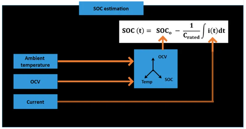
The above is a generalized form of how a BMS works for SOC estimation. Depending on the method used for SOC estimation various parameters are taken as input by the BMS. These parameters are used further to calculate the SOC using various relations as per the method and SOC is given at the output. In our case temperature is not needed since the Coulomb counting method is independent of the working temperature of the battery.

Modified Coulomb Counting Method

To improve the Coulomb counting method, a new technique called modified Coulomb counting method is proposed. The modified Coulomb counting method uses the corrected current to improve the accuracy of estimation.

The corrected current is the function of discharging current. There is a quadratic relationship between the corrected current and discharging current of battery. By practice of experimental data, corrected current is calculated by the following form:

`I_c(t) = k_2I(t) 2 + k_1I (t) + k_0`

where , and are constant values obtained from the practice experimental data.

In modified Coulomb counting method, SOC is calculated by the following equation:

``SOC(𝑡) = SOC(𝑡−1) + 𝐼𝑐 (𝑡) / 𝑄𝑛 *dt``

The experimental results show that the accuracy of the modified Coulomb counting method is superior to the conventional Coulomb counting method.