Week 7 State of charge estimation

https://in.mathworks.com/matlabcentral/fileexchange/72865-design-and-test-lithium-ion-battery-management-algorithms

1.Simulate the 3 test cases from harness dashboard and write a detailed report on the results

2.What is coulomb counting? Refer to the above model and explain how BMS implements coulomb counting for SOC estimation ? 

Hint :(Download the file from the link and go to SOC estimation model-ECU block)

    

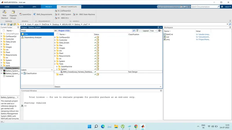
After this the BMS_ClosedLoop_Harness_Dashboard model file is open as:-

    

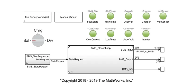
 Block of Model:-

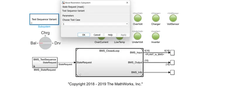
• Test sequence Variant (it has 3 different test condition)
• Manual Variant (selection)
• BMS_StateRequest subsytem to provide the state request commands.
• Indictaing lamps are there to show any fault state, High Temp, Overvoltage, Charger, Voltage Sensor, Overcurrent, Low temp, Under Voltage, Inverter state of  a battery. Green light tell us that all states are Ok and battery is good to charge and discharge and red indication will indicate the fault state.
• Rotating switch for manual variant to change the position during simulation run time
• BMS_Closed Loop:- this subsystem contain BMS ECU and Plant as two main subsytem and lets see this block in details:-

     

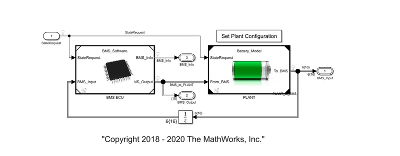
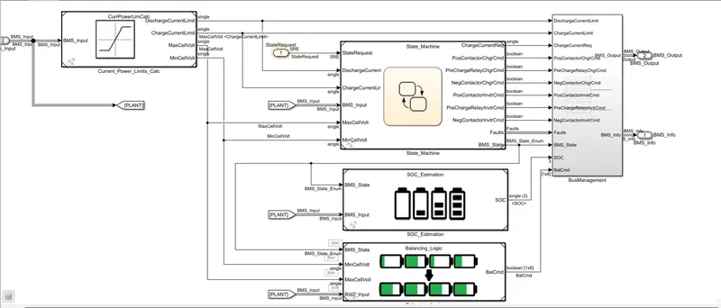
BMS ECU:- The BMS ECU get have two input which are BMS_Input which is feedaback from the Plant model and The state Request is coming from the state machine . This is generating output as BMS Output and Info which have current power limit calculation in State Machine, SOC estimation and Cell balancing logic as shown below:-

 

 Plant:- This subsytem contain Battery pack, precharge circuit and charger / loads. In the battery pack there are two configuration which are 1 module (6 cells) and 16 module (96 cells). Here we have selected 1 module for simple calaulation and less simulation time.

 

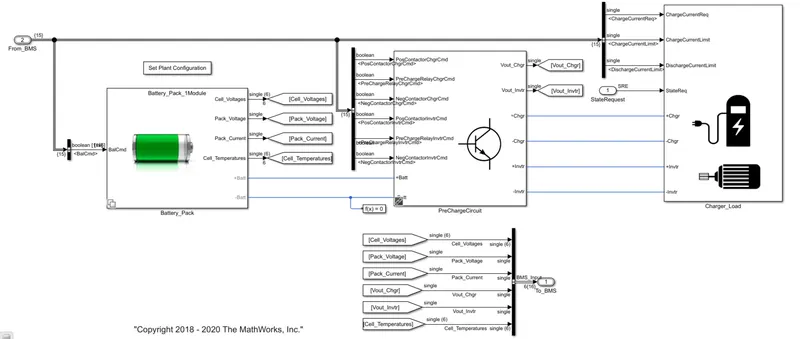
• In the scope SOC of module, Cell voltages, Pack Current, Cell Temperature, BMS state and cell balancing command are seen as output.

Task:- 1.Simulate the 3 test cases from harness dashboard and write a detailed report on the results

For simulating the three test cases we have to go to the Test sequence Vaeiant and select there Test Case one by one.

We can see the Test sequence in BMS_StateRequest>BMS_TestSequenece and there we can see that the test case we have selected is as shown below:-

• Output results

    

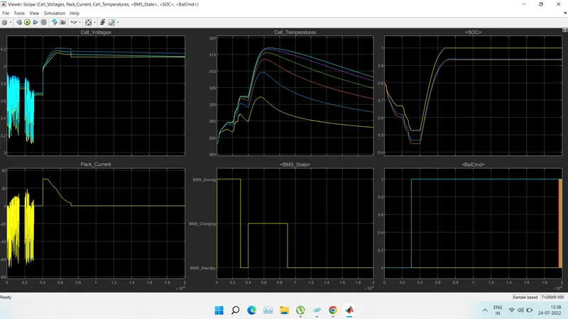
                                              Fig- Result plots

i) Driving (Discharging) mode (0-3000 sec):- All the cells for the first 3000 sec are in driving mode so the dicharge of all the cell occurs and its varies in the range of 3.1 to 3.9 V (min and max.).

Cell temprature increases from 288K to 302 K.

SOC also reduces from 80 % to 45% for EKF technique.

ii) Balancing mode (3000-4000 sec) :- After 3000sec for 1000 sec, cell balancing occur and the Modules are in standby mode and they are having constant voltage near about 3.7V.

Cell temperature reduces slowly as no current flow through the cells during balancing.

SOC is also constant during this period i.e. 45% for EKF technique.

iii) Charging and Balancing (4000- 9000 sec):- After 4000 sec the charging occurs and the cell voltages increased from 3.7 to nearly about 4.2 V in Constant current mode with current of nearly 30A and then the constant voltage charging starts and current reduces from 30A to 2.6 A Charging and balancing of cells occur till 9000 sec.

Cell temperature also start to increase exponentially upto constant current region and reduces as current flow reduces in constant voltage mode.

SOC also increases from 45% to 94% in this mode for EKF technique.

iv) Post charge Balancing (9000- 20000sec):- After 9000 sec the post cell balancing starts under standby mode.

Cell temperature reduces in this mode and tries to reach the ambient temperature.

SOC remains constant to 94%.

• Test 2

Simulation is ran for 20000 sec and the result are as below

   

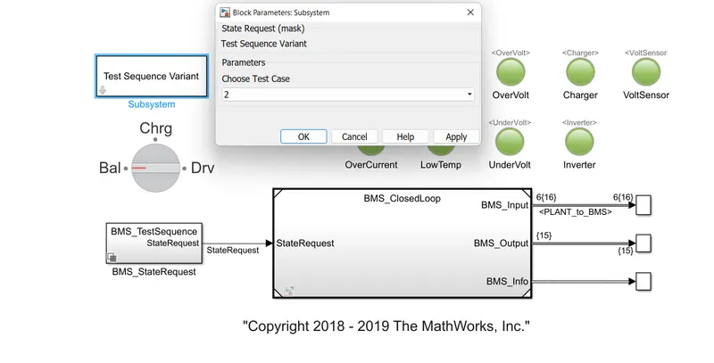
 The editor figure tell us about the test sequence and it is as following:-

• Driving is done for first 10000 sec.
• Then Charging is done for next 10000 sec.

• Simulation is ran for 20000 sec and the result are as below:-

    

The Lamp indication were green for all states which means the model is fault free.

The test rsults are shown below of test 2

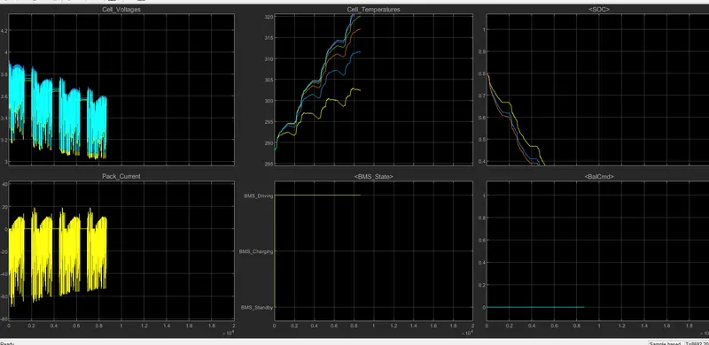
                                                       Fig- Test plots 2

i) Driving Mode (0-10000 sec):- The cell voltage varies from 3.9 V to 3.05 volt ehich is cut off voltage of cell and the entire cell is drained upto 8692 sec.

Cell temperatures varies from 288K to 322.5K.

SOC reduces from 80% to 0% (cell got fully drained) in the drive mode under 8692 sec.

     

Cell balancing is not performed here.

ii) Charging Mode (10000- 20000 sec): The cell got drained earlier before reacching this mode

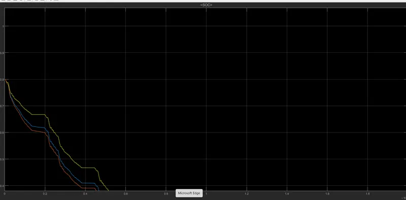
Initially the state of charge of battery module is in 80%. 

Here the yellow plot represents SOC estimation done by coulomb counting technique.

Blue plot represents SOC estimation using Unscented Kalman filter technique.

Red plot represents SOC estimation using Extended Kalman filter technique. Among three UKF and EKF techniques estimate accurately than coulomb counting technique.

Initially for 3000 secs SOC decreases to nearly 45% during drive mode.

After 3000secs upto 4000 secs the SOC is constant at 45%  as cell balancing occurs in standby mode.

From 4000 secs to 9000secs module in charging mode.(4000 to 7000=CC mode,7000 to 9000=CV mode).

After 9000 secs the SOC becomes constant approximately 94%  as seen from above plots.

c) Test case- 3

The test case 3 is selected as shown below in the dialog box and click OK to implement it.

          

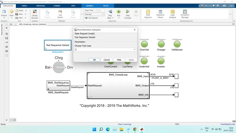
                                                       Fig-Test select 3

The test case 3 is selected as shown below in the dialog box and click OK to implement it.

       

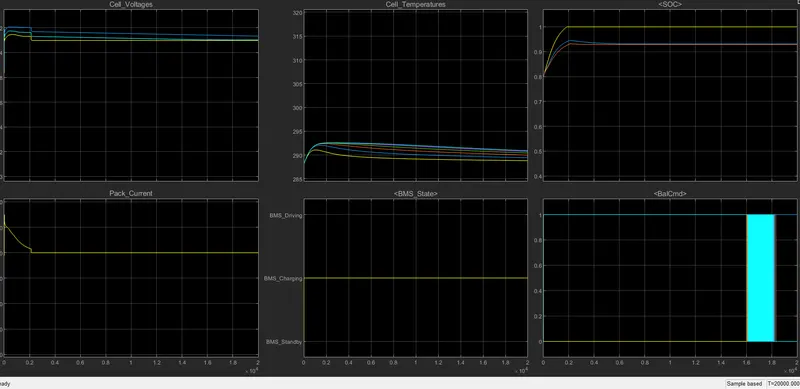
                                                          Fig-Test plots 3

• SOC plots 3

                 

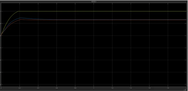
                                                     Fig-soc plots

i) Charging (0-20000 sec):- Cell Voltages increases from there intial values and after 2000 sec they got constant .

Pack current initally start from 0 to 30A and then start decreasing when the constant voltage mode is there to 2.5 A and got full charged upto 2000 sec.

SOC was initally 80% and in 2000 sec it got fully charged that is 100%.

Cell temperature starts to incraeses initally and when battery got fully charged then decrease down to the ambient temperature.

• Temp output

   

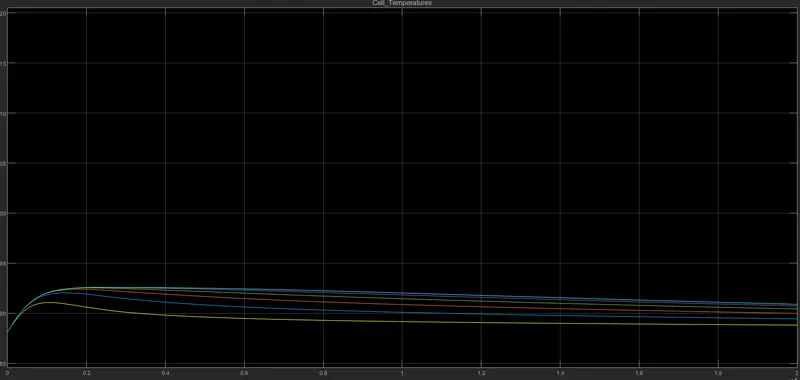
The cell temperatures continue to increase heat upto full charge and after that the temperatures get started to reduces to ambient temperature.

As shown from result plot the temperatures start decreases after full charge(at 2000 secs).

• Voltage output

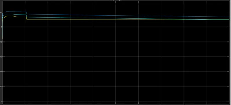
Initially cell 2 , voltages rises from 3.9V(approx) to maximum 4.2V and stabilised to 4.15V. Cell 1 reises from 3.85V to 4.1V and stabilised to 4.08V. The battery pack current raising from 0A to 30A and starts to  reduce to 2.5 A gradually at end of full charging upto 2000 secs. At 2000secs the pack is fully charged to 100%.  After full charge current flow will be cutoff  as shown in result plot.

 Here from 0sec the cell 6 and 2 starts to balance with respect to cell 1 and all cells are try to balancing at end of simulation.

• Conclusion:

Hence from above three test cases the performance of BMS on various factors are discussed and analysed.

B)To explain coulomb counting for finding the SOC estimation in BMS. 

Coulomb counting:

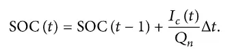
SOC(State Of Charge) is defined as the rate of available capacity to its maximum capacity when a battery is fully charged and describes the remaining percentage of the battery

capacity.

To find this SOC % we are using coulomb counting method.

The coulomb counting method measures the discharging current of the battery and integrates the discharging current over time in order to estimate SOC.

Which can be estimated from discharrging current(I(t)),previously estimated SOC values(SOC(t-1)).The relation can be given as,

Modified Coulomd counting:

In this technidue discharge current is corrected with a function and corrected current is found out for accurate SOC estimation.

The function can be given as,

Where K0,K1,K2 are constant values obtained from the practice experimental data.

The SOC relation can be given as,

SOC estimation in BMS model:

To see the model of coulomb counting technique in BMS model click the subsystem of SOC_Estimation and click Coulomb counting.

     

                             

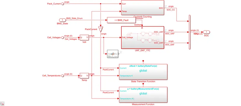
It is developed as shown below,

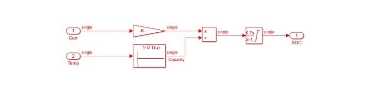
Here the discharge current from battery given to gain with value as 1/3600 to convert current to Ahr.

The value is divided by capacity due to temperature change. Then integrated with a gain value of 1 with sample time -1 as we are using discrete integrator.

The saturation limits are from 0 to 1.

We will get the SOC values from 0 to 1 multiplied with 100 to get in percentage of SOC. 

       

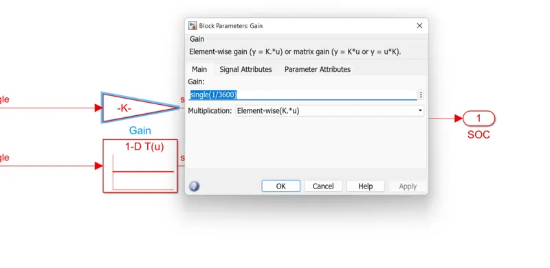
Here the discharge current from battery given to gain with value as 1/3600 to convert current to Ahr.

The value is divided by capacity due to temperature change. Then integrated with a gain value of 1 with sample time -1 as we are using discrete integrator.

The saturation limits are from 0 to 1.

We will get the SOC values from 0 to 1 multiplied with 100 to get in percentage of SOC. 

      

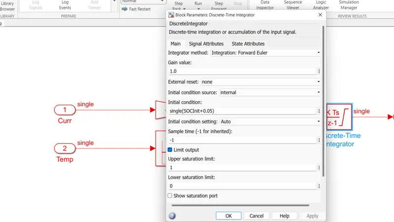
 That current is divided by the capacity due to temperature change and then intregrated with the gain value of -1  wo=ith sample time of -1 as discrete type integrator is used here. 

The saturation limits are given which are 1 to 0. So that we get the SOC value  from 0 to 1 multiplied with 100 to get percentage of SOC.

This Coulomb Counting methos is simple and require less computational compared to other two methods