Week 7 State of charge estimation

Aim:Simulate the 3 test cases from harness dashboard and write a detailed report on the results

We have to extract the file from the downloaded zip folder,from the battery model,we have to open the BMS system and closed harness dashboard,We can see the closed harness dashboard below,

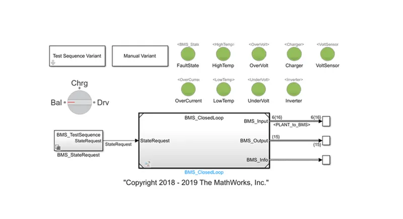
In this model,we can see the Test sequence variant subsystem which consists of 3 different test cases,and the green light indicates the system is working perfectly,and the red light represents errors in the system.

We have to proceed the 3 test conditions in the BMS test sequence ,for that first we have to choose the test 1 sequence from the Test Sequence Variant subsystem,

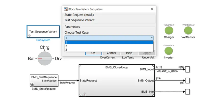
From the BMS_StaeRequest we have to select the testSequence1

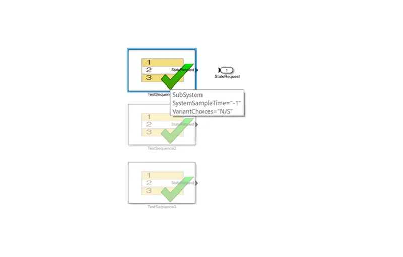
The table below shows the properties of the testsequence1

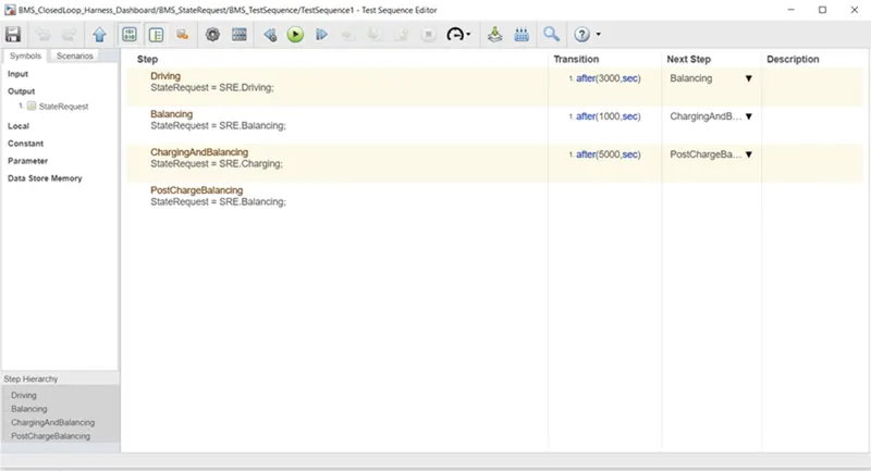
• The first condition is Driving and is set for 3000 seconds
• The second stage is balancing and the duration is 1000seconds
• The third condition is ChargingAndBalancing where it is ran for 5000 seconds
• After that we have post charge balancing till the end of the simulation.

Now we have to simulate the model and examine the results,

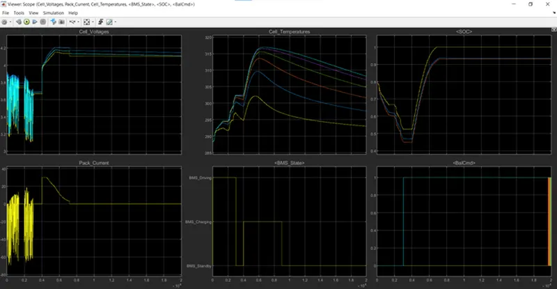
From the Cell Voltage graph we can see the voltage varies from 3.2V to 3.9V depending on the driving mode, we can see the variation depending on system output, after 3000s the voltage always goes to the next phase of form 3000 to 4000, where the wait occurs 1000 seconds in the measuring phase, the third mode of charging and measuring, where the voltage graph shows a sudden increase of form 3.7V to 4.2V, and after that we see a slight decrease in the decrease of 4.1V, and in the case of background charging voltage it moves at a constant rate until the end of the simulation.

From the cell temperature graph the initial temperature is 288K and gradually all 6 temperatures rise the first cell temperature rises to 298K and the 6th cell reaches a range of 302K. this is the scope of the first drive. in the second stable case we can see the temperature drop by a small distance to 298K in the first cell and after 1000 years the temperature has a noticeable rise to 318K in the 6th cell and 302K in the first. cell.In the case of post charge we can see graph reduction, in the sixth cell it is 308K and in the first cell it is almost 292K at the end of the match.

In the SoC graph we have the first SoC is 80% and in the case of the drive cycle it falls to 45% of the 6th cell and 55% of the first cell, And the next conditon balances when the graph reaches the standby mode of 1000s and in the next cycle of charging and balancing we can see a sudden increase in SOC up to 100% and 92% keeping the same amount of post charges constant until the end of the match.

From the current package graph we can see in the current drive mode it varies from the 10A and -70A pack values ​​and the frequency is also high at 3000s and when in the second mode, it achieves the standby mode for measuring cells. and fluctuations can be seen from 8A to 65A and proceed to the next stage a sudden rise can be seen up to 30A value and gradually decreases until the end of the stage.In the case of post charging continuous always keeps the value zero.

In the BMS status graph in the driving section we see that it is initially in the driving mode for 3000s years, In the next section it shows the positioning position of the 1000s cell balance, and after that it reaches the charging mode of 5000s and moves. waiting until the end of the simulation.

In measurement cells, we can see cell 6 rise from zero to 1 behind the drive stage, but cell 1 shows the continuous value of all 3 stage conditions and in the charge mode of transmission cells reach the same number.

Test case 2

we have select the test 2 sequence from the Test Sequence Variant subsystem,

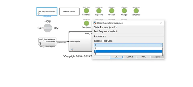
From the BMS_StateRequest we have to select the testSequence2

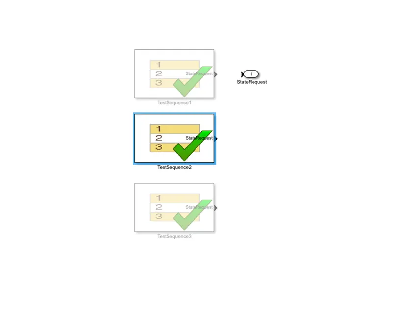
The table below shows the properties of the testsequence2

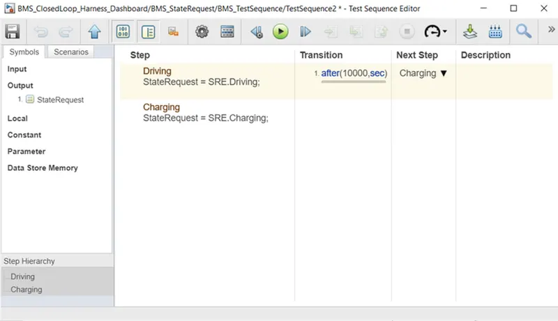
From the test properties,the test sequence consist of 2 stages,Driving and charging ,the simulation is done for 20000 seconds. We can examine the results,

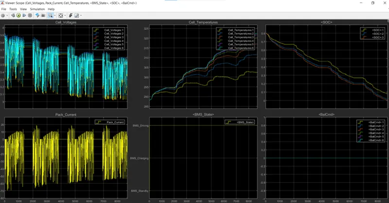
From the cell voltage graph we can see that up to 9000 seconds, cell volumes range from 3.9V to 3.05V as high as cutoff voltage. it's over.

In the cell temperature graph we can see the temperature rise from 288K to 322K, Cell 1 has low temperature fluctuations, ranging from 288K to about 302.5K. Cell 6 has a high temperature range, ranging from 288K to about 322.5 K. the length is in the standby mode, the cell temperature drops slightly between driving modes.

We can see variations in the SOC graph, the initial level is 80% and gradually decreases with time.In full drive mode, as shown in the article above, the SOC drops from 80% to 0% (currently long-term output). SOC remains the same in the waiting conditions between them.The original cell does not reach the zero value at the end of the simulation period.

In the current pack of the pack, it currently varies from the 10A and -70A value of the pack and the frequency is also high. Between driving modes, there are certain standby mode conditions.

In BMS status graph the graph only shows that it works in driving mode.The graph changes from standby mode to driving mode until the end of the simulation period.

In the cell measurement graph shows the zero value by measurement.

Test case 3-

For simulating the third case We have to select the test 3 sequence from the Test Sequence Variant subsystem,

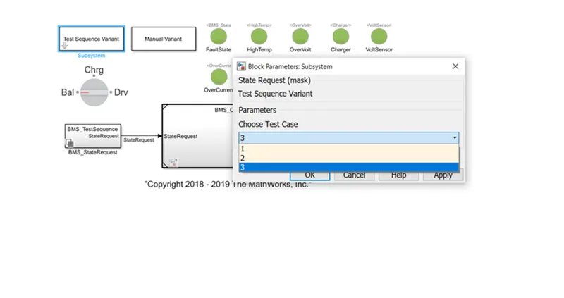
From the BMS_StateRequest block we have to select the testSequence3

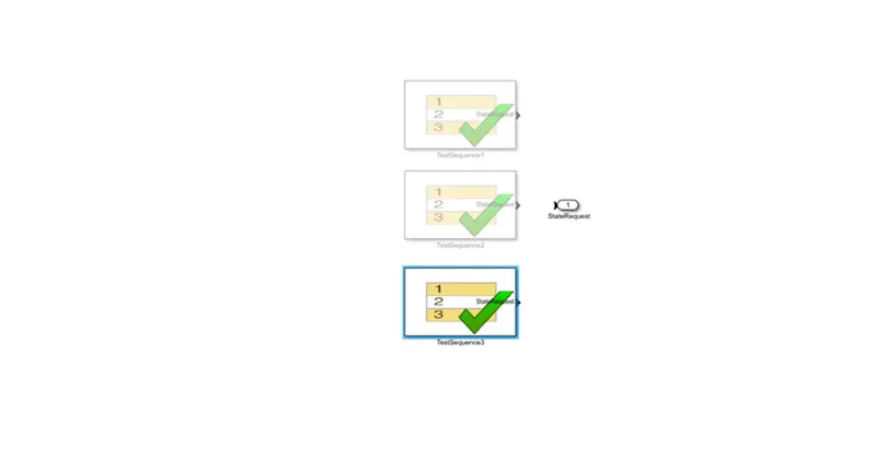
The table below shows the properties of the testsequence3

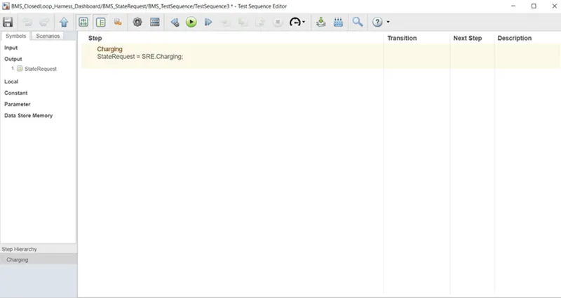
In this case we have only one stage that is charging for the complete simulation time.We can see the plots below,

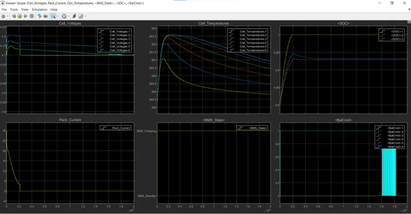
From the cell voltage graph we can see that initially, the voltage in cell 2 rises from 3.9V to 4.2V before the stability of 4.15V. After 2000 seconds we can see the graph go down the line to the end of the simulation. Cell 1 goes from 3.85V to 4.1V and stays at 4.08V.

In the cell temperature graph, initially there is a sudden increase in cell temperature, from 288K to 292.5K and decreases significantly to the end of the simulation.

In the SOC graph we can see an increase in SOC scope, from 80% to 100% cell 1 becomes the highest value and ceel 2 and 3 reaches a total of 92.5% and remains at that value until the end of the simulation.

In the current package graph, we can see a sudden drop from 30 to 0. The graph reaches zero in the 2000s and goes on and on until the end of the simulation.

In the case of BMS we can see the graph moving in charging mode and in measuring the cell graph, cell 1 balances during simulation.

2.What is coulomb counting? Refer to the above model and explain how BMS implements coulomb counting for SOC estimation ?

Ans-

The Coulomb calculation is a way to track the Charging Status of a battery pack. Calculates the total amount of energy coming in or out of the battery pocket by combining the active flow energy (measured by amps) over time. This results in a volume that is usually expressed during Amp-hours,

When the battery is fully charged, the SOC (State Of Charge) is defined as the average available capacity to a maximum capacity, and indicates the remaining percentage of battery capacity. The coulomb calculation method is used to calculate the percentage of SOC.
To measure SOC, the coulomb calculation method analyzes outgoing battery power and incorporates charging over time. Calculations using output power (I (t)) and pre-calculated SOC values ​​(SOC (t-1)). Relationships can be described as follows,

SOC=SOC(t−1)I(t)Qn△tSOC=SOC(t-1)I(t)Qn△t

In modified coulomb counting the discharge current is corrected with a function and corrected current is used for SOC calculation,we can write the equation as,

Ic(t)=K2I(t)2+K1I(t)+K0Ic(t)=K2I(t)2+K1I(t)+K0

And SOC equation can be written as,

SOC(t)=SOC(t−1)+Ic(t)Qn△tSOC(t)=SOC(t-1)+Ic(t)Qn△t

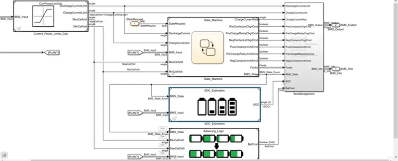
We have the Coulomb counting technique in the BMS model,so we look into the SOC estimation subsystem,

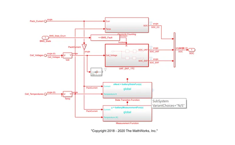
In the coulomb counting susbsytem,we have the configuration as shown below,

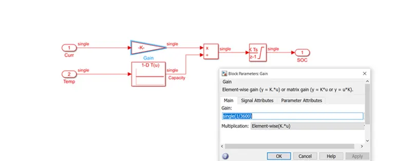
To convert current to Ahr, the discharge current from the battery is given to gain with a value of 1/3600.Temperature changes cause the value to be split by capacity.

Then, because we're using a discrete integrator, we'll integrate with a gain of 1 and a sample time of -1.

Saturation thresholds range from 0 to 1.We'll multiply the SOC values from 0 to 1 by 100 to get a percentage of SOC.