Week 7 State of charge estimation
Solution 1:
Test case 1:
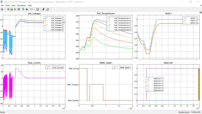
It involves Driving cycle for 3000secs and about 500sec of standby followed by charging cycle from 4000-9000seconds.
Plot-1 (Cell Voltage) depicts the cell voltage patterns initially for the period in which BMS is in driving mode, so there is a fluctuation in all the cell voltage depends upon the input drive cycle signal. After 4000secs it shows continuous gain in all the cell voltages as it is subjected to charging mode.
Plot-2 (Pack Current) depicts the equivalent output cuurent in positive and negative range meaning charging and discharging depends on the input signals, after 9000secs because it is in standby mode it remains at 0
Plot-3 (Cell Temperature) depicts there is gradual rise in the temperature during driving with a sudden fall during the small standby period and gradual rise during the charging mode, then it stabilizes due to standby mode as well as through heat transfer through convection.
Plot-4 (BMS State) depicts the different modes and its activation duration
Plot-5 (SOC) SOC drop during the initial driving mode and it rises because of charging mode.
Plot-6 (Balance Command) Active balancing is employed in the model which enables the excessively available charge to the cell which is yet to reach its maximum capacity
Test case 2:
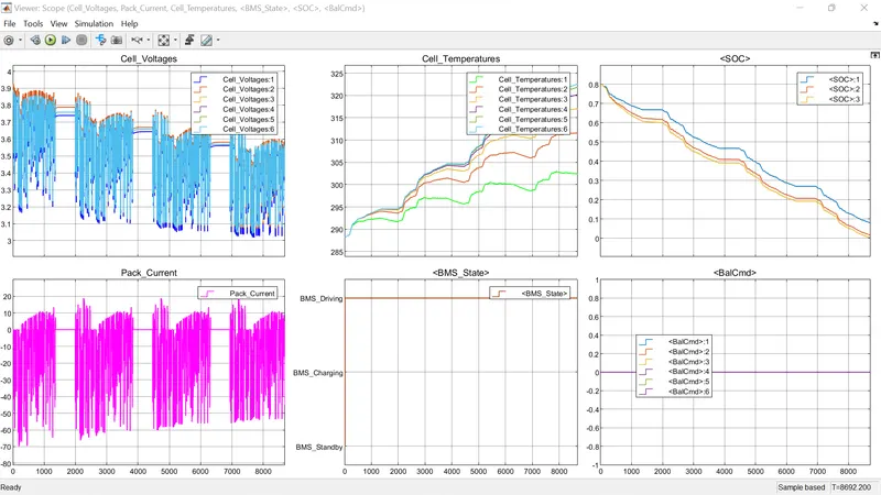
It involves Driving cycle for the whole simulation time.
Plot-1 (Cell Voltage) depicts the cell voltage patterns for concerned drive cycle signals as it is getting drained the cell voltages are approching its cut-off voltage at the end of 8000seconds
Plot-2 (Pack Current) depicts the equivalent output cuurent in positive and negative range meaning charging and discharging depends on the input signals, after 8000secs it is stopped because the battery got drained completely
Plot-3 (Cell Temperature) depicts there is gradual rise in the temperature all the driving cycle beacuse of discharging a lot of energy for about 8000seconds continously, leading to a temperature above 300K in all the cells.
Plot-4 (BMS State) depicts the drivingt mode activation duration
Plot-5 (SOC) SOC drops towards zero as it is getting drained by the driving cycle due to which it approched 0% SOC at 8500 secs
Plot-6 (Balance Command) As this case invloves no charging thereby depicts no Balance command in plot
Test case 3:
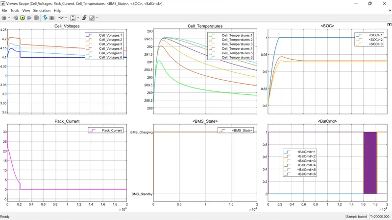
It involves Charging cycle for the whole simulation time.
Plot-1 (Cell Voltage) depicts the initial cell voltage rise and stabilization for the rest of the simulation time.
Plot-2 (Pack Current) depicts the pack current is zero because of no driving cycle has been applied to the battery pack.
Plot-3 (Cell Temperature) depicts there is gradual rise and then it stabilizes due to heat transfer through convection.
Plot-4 (BMS State) depicts the charging mode activation duration
Plot-5 (SOC) SOC rises and approaches because of charging mode.
Plot-6 (Balance Command) Active balancing is employed in the model which enables the excessively available charge to the cell which is yet to reach its maximum capacity
Solution 2:
2.1 Coulomb Counting:
It is one of the way to determine the SOC of a cell in a battery pack. It is calculated by integrating the discharge current over the time and dividing it by it's capacity. Then this value is deducted from the previous SOC value and the procedure repeats.
SOC(t) = 1/C∫I(t)dt
C- Capacity I - Discharge Current
2.2 Implementation of Coulomb counting in BMS:
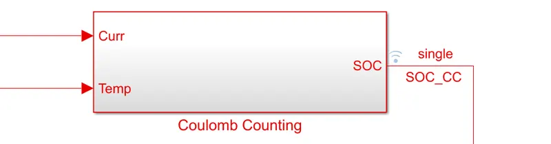
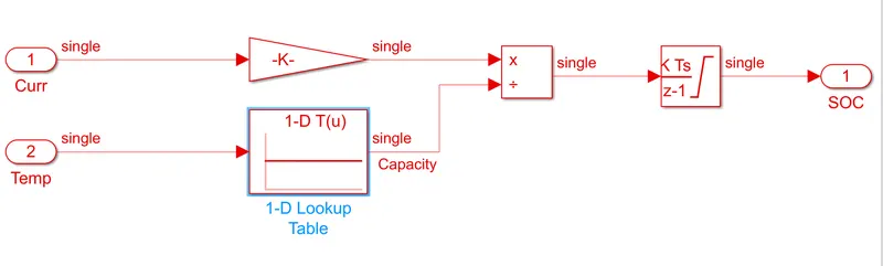
In BMS system the following steps are followed
1. Two inputs are given namely current and Temperature of each cells.
2. Current is then given to the gain block where [(1/3600) * Current] is performed.
3. Temperature and Capacity is plotted as 1-D graph to determine the capacity at different temperatures.
4. Output of Gain block is divided by the Capacity value.
5. Integrator block performs the integration opearation over the simulation time.
5. Final output will be the SOC of the cells.