Week 7 State of charge estimation
1.Simulate the 3 test cases from harness dashboard and write a detailed report on the results.
The BMS model consists of BMS ECU (Electronic control unit) and a plant. The BMS system provides functionalities to control the battery pack. the control unit with its various monitoring and control algorithms is connected to a block with a representation of battery pack.
This is the BMS implemented in MATLAB along with the battery pack.
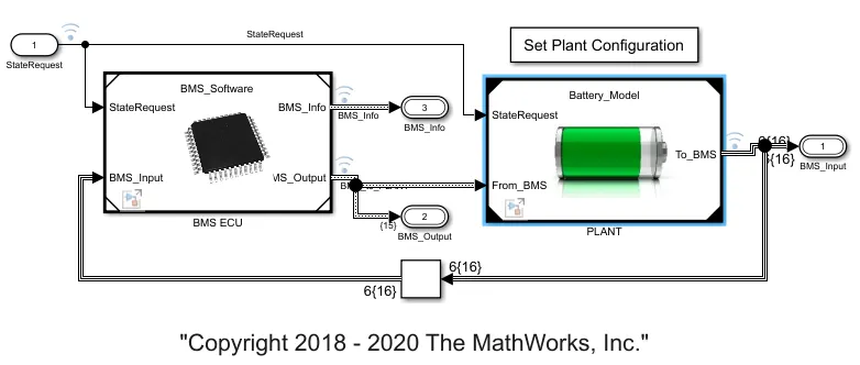
From the above MATLAB model we are simulating 3 test sequences from harness dashboard to find out the fault condition in BMS.
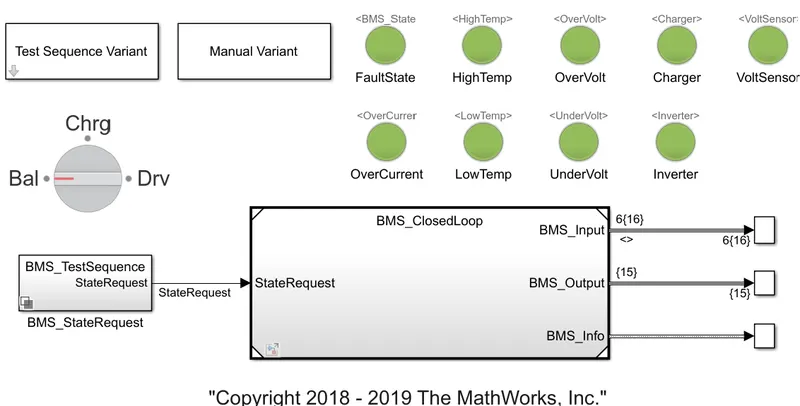
The Below model shows the dashboard wherenwe can get the information related to the faults like over voltage, high temperature, over current and inverter related faults. If there is any fault conditions the indicators will blow in red light colour otherwise it shows green indicator means no fault.
The state machine in the BMS ECU defines the main operating state of BMS.The state machine has four parallel states:
1. Thre firsyt one defines the variable BMS state which indicates standby, driving, charging, and fault. Charging comprises constant current and constant voltage stages.
2. The second state switches the fault state ON in case a current, voltage, and temperature value reaches an unsafe level.
3. The third and fourth states define the contactor ON and OFF awitching sequence for charger and inverter.
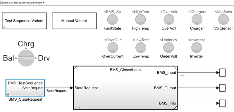
The harness dashboard is used to control and identify the test sequence states in the state machine. It consists of the test sequence varient subsystem which hold three different test cases.
Test Sequence-1 Drive-Balance-Charge:
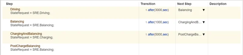
When simulation begins, initially the vehicle is driving state and the SOC will decrease for this time period of 3000 seconds. The next step is balancing mode and the vehicle is in standby condition in time period of 1000 seconds. After that the vehicle is in the charging phase and the battery SOC is incerase in 100%. The next phase is the post charging phase in which the vehicle again goes by the standby mode.
Result:
1. The input cycle seen in the BMS state plot in which the vehicle initially undergoes driving, then charging till SOC = 90% and then later in the standby mode.
2. During charging the battery pack voltage is increased upto 4.2V.
3. The SOC drops to less than 50% after drive cycle and than later give it to charging until SOC reaches 100%.
4. The current supplied to the EV during the driving phase can be seen in the current plot.
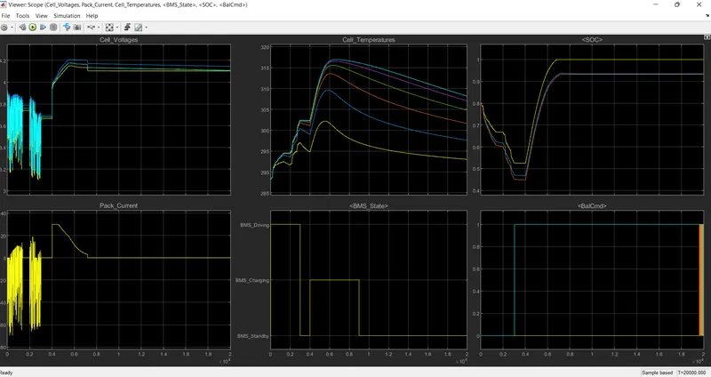
Hence, there is no fault observed from the dashboard.
Test Sequence - 2 Driving-Charging:
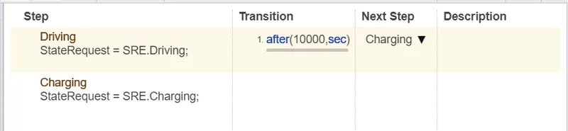
Result:
1. Discharging mode/ BMS driving at time instant 0 till the end of simulation.
2. Cell voltage reduced from initial 4 V.
3. Pack current reduced to 0.
4. SOC is initially of 80% and reduced to 0%.
5. Cell temperatures increased from 289.15 to maximum recorded from 323k and differences in incerase 33k this increase is different and comparatively less with maximum recorded as 323k for other output graphs.
6. Cell balancing is ideal in this time period.
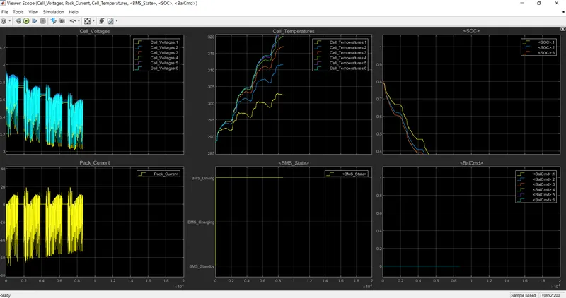
Hence, there is no fault observe from dashboard.
Test Sequence - 3 Charging:

Result:
1. Cell voltages and pack current combine we can observe the constant current (CC) and constant voltage (CV) characteristics of a battery pack. from initially time period of 0 sec the cell current increased to 30 Ah and cell voltage is also reached to 4.2 V this phase of operation is called constant current.
2. SOC is initially of 80% at time instant of 0.2 sec this is increased to 100% or 1 to its full capacity.
3. Coulomb counting: From the result the yellow graph showing this method where the SOC is reached to 100% at time of 0.2 sec.
4. UKF and EKF Kalman filter: Both SOC estimation from this method is 93%.
5. Cell Temperature is increased from initially 288 to maximum recorded as 292.5 with difference in temperature rise is recorded with other cell Temperature estimation graph.
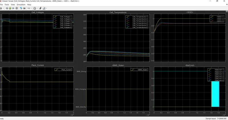
Hence there is no fault observed from dashboard.
2.What is coulomb counting? Refer to the above model and explain how BMS implements coulomb counting for SOC estimation ?
The “coulomb counting” or CoulCount method was developed by Schmitt . as a heuristic method, although the underlying theory is reasonably accessible . It depends on the recording of the current noise only. The signal is filtered with a high-pass filter with a cut-off frequency of 0.01 Hz. The filter may be either analogue (although the implementation of a good-quality 0.01 Hz analogue filter is difficult) or digital. The absolute value of the measured current samples is then summed over time. A steep slope is taken as an indication of rapid corrosion, although it is not possible to calibrate this in terms of an estimated corrosion rate.
To determine available capacity, coulomb counting relies on the integration of the current drawn from and supplied to a battery over time, τ∈t0t, as given by
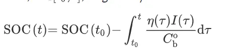
where I is the current and η is the efficiency during charge and discharge operations . Coulomb counting is advantageous in terms of a simple structure and its ease of implementation. However, some problems make it difficult to accurately estimate battery SOC by coulomb counting. Because battery capacity and efficiency are significantly influenced by operating temperature and current direction, these factors should be considered to correct for battery SOC. Sensor accuracy is also important because accumulated errors can lead to a drift in the estimated battery SOC. Furthermore, one of the main problems in coulomb counting is that it is necessary to calibrate the initial battery SOC. In several applications, the initialization involves rest and the initial SOC is estimated based on the voltage inversion method described next.
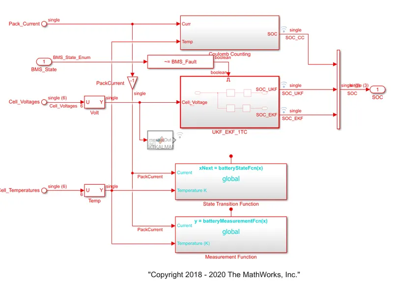
Coulomb Counting Method:
The Coulomb counting method is associated with monitoring the input and the output current continuously. Since capacity is the integral of current with respect to time, by measuring the input and the output current, change in capacity or capacity degradation of a battery can be measuredeasily.In this method,So His calculated by dividingm easured capacity (after discharging the battery to 0% SoC value).
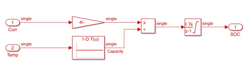
Coulombic Efficiency: For a given battery, the releasable charge is always less than the stored charge during an operation cycle. This effect is denoted as the Coulombic efficiency (ߟ ,(by which the current in the Ah method is usually multiplied as a correction. The calibration of ߟ is complex because both temperature and current rate influence it . ߟ is near 1 at low rates and declines at high rates due to the significant internal loss by secondary reactions. Kong et al. investigated the correlation between ߟ and SoC. However, they only focused on the variable discharging rates with the charging rate fixed and the influence of temperature ignored. considered current rate and temperature based on a large measurement matrix of different rates and temperatures to cover all possible operating conditions.
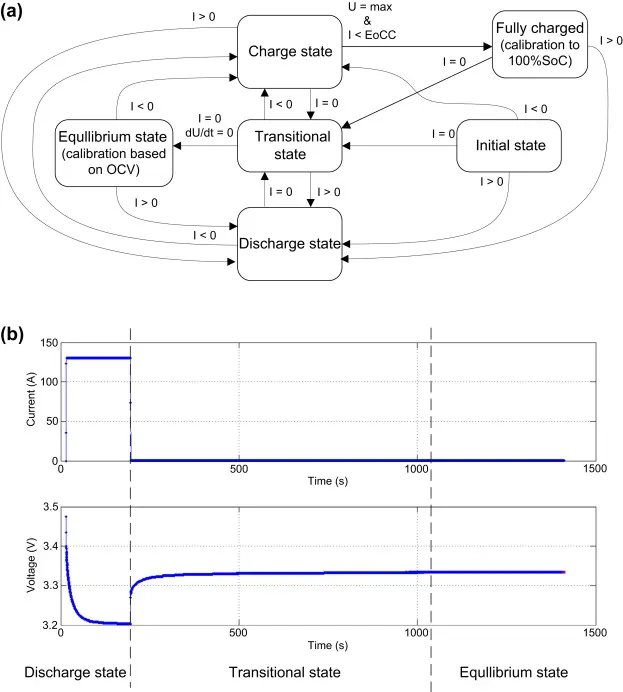
An illustrative state diagram of this method is shown in fig. A cell or battery can be in one of six states. A change of the state is detected by monitoring voltage and current. The coulomb counting method is used in almost all states with exception of “Equilibrium state” and “Fully charged”. In equilibrium state, the battery voltage is stable and OCV voltage characteristic is used to calibrate the state-of-charge. A calibration is also done when the cell is fully charged because this state is well determined and easy to detect during the constant-voltage charging mode. In this mode, a maximum voltage is applied to the battery and current decreases with time. When the current reaches a minimal value, defined as end of charging current (EoCC), the charging process is complete and the battery is fully charged. An example of cell voltage and current in three different states is shown in Figure.
The battery capacity decreases with age and cycling. Therefore, the reference value of nominal capacity also needs a periodical calibration. The easiest way is to perform a full charge and discharge cycle at low current rate (reference cycle). Based on this cycle, a discharge capacity is measured and a maximum capacity value is updated.
This method is of relatively simple implementation and gives good accuracy. An estimation error of this method using a little more sophisticated algorithm was reported to be lower than 3% during full cell cycling. A drawback is that an SoC estimation error can still increase to significant values if a battery is used continuously and resting times between charge and discharge cycles are not long enough to reach voltage equilibrium and perform calibration.
State of Charge
SoC determination depends on the cell chemistry. In most cell chemistries, the reversible cell voltage depends on the SoC. The voltage difference between the fully charged cell and a discharged cell can be more than 0.5 V. The cell voltage (at open circuit or at low charge and discharge currents) is a useful measure of the SoC. For chemistries with a small dependence of voltage on SoC, techniques such as coulomb counting have to be employed. If lithium-ion batteries are not frequently fully discharged and recharged (deep-cycled), the recalibration of some external electronic fuel gauge, e.g., an SoC meter, might require a deep cycle after about every thirtieth recharge to prevent the display of incorrect battery charge.
Reversible Cell Voltage
The reversible cell voltage E0 or electromotive force of the cell in the electrochemical equilibrium, calculated from thermodynamic data, or the OCV U0, by practical measurements, is the driving force for electricity generation in a battery. It is a function of the SoC and therefore can be used as an accurate fuel gauge.