Week-4 Challenge WOT Condition Part-2

1. What is the difference between mapped and dynamic model of engine, motor and generator? How can you change model type?

Aim: To study the Powertrain block set in Matlab

Theory: Powertrain Blockset provides a set of fully assembled reference applications, including gasoline (spark-ignition, SI), diesel (compression-ignition, CI), hybrid, and electric vehicle systems, as a starting point for your powertrain system model. Powertrain Blockset provides two types of combustion engine models: mapped and dynamic. Mapped engines represent macro engine behavior as a set of lookup tables (brake torque, fuel flow, air mass flow, exhaust temperature, efficiency, and emissions) as functions of commanded load and measured engine speed. Dynamic engines decompose engine behavior into individual component models that account for engine dynamics, most notably intake airflow and turbocharger dynamics.

You can switch between engine model types based on your application. Dynamic engine models are suitable for designing control, estimator, and diagnostic algorithms that depend on dynamic subsystem states, for example, in closed-loop AFR control algorithm development. Mapped engine models are suitable for analysis and design activities that do not require engine subsystem dynamic characteristics, for example, in engine and transmission powertrain matching analysis for fuel economy, emissions, and performance tradeoffs.

Mapped Model:

Model uses a set of steady state lookup tables to characterize engine performance. If you have engine data from a dynamometer or design tool like GT-POWER.

The tables provide overall engine characteristics, including actual torque, fuel flow rate, BSFC and engine out exhaust emissions. For quasi steady state engine simulations.

The mapped motor and drive electronics operating in torque control mode. The output torque tracks the torque reference demand and includes a motor- responce and drive responce time constant. electric losses need to be specified if present.

Dynamic Model:

Model decomposes the engine behaviour into engine characteristics that are seperated in to lower-level components. By combining components in this way, the model capture the dynamic effects. If you need a more detailed dynamic model and have component level data. To analyze the impact of individual engine components on the overall performance.

It contains interior PM controller, three phase voltage source inverter and internal permanent magnet synchronous machine (PMSM). All these combination given EV dynamic. Parameters of motor, current, electrical, etc are given.

Changing Model Type:

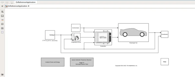
Open 'EV Reference Application' in powertrain blockset of MATLAB as shown in figure below it. It is simulink Model which consists of Drive cycle, Envinorment conditions, Longitudinal driver controllers and passenger car.

Now open the passenger car block and select the electric plant.

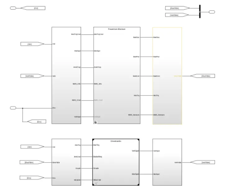
After selecting electric plant and then select 'MotGenEVMapped' block.

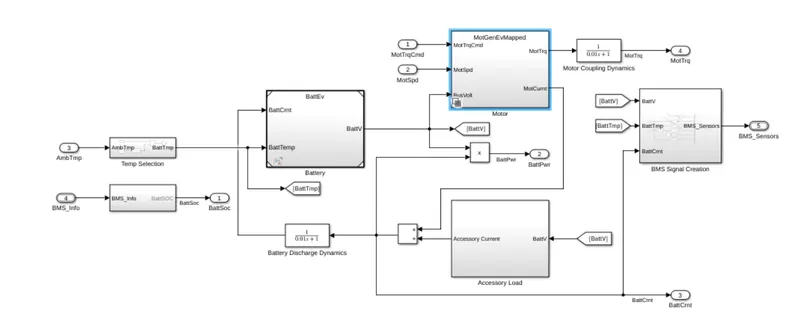
From the below figure it is clear that by defalut mapped motor is selected.

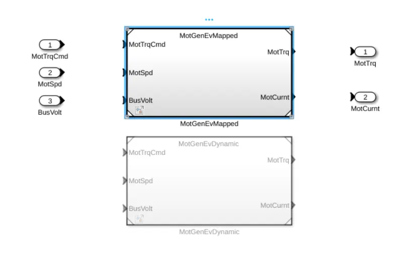
Now changing the mapped to dynamic block set, right on the screen and select 'Varient'. The select Label Mode Active Choice and select "MotGenEVMapped".

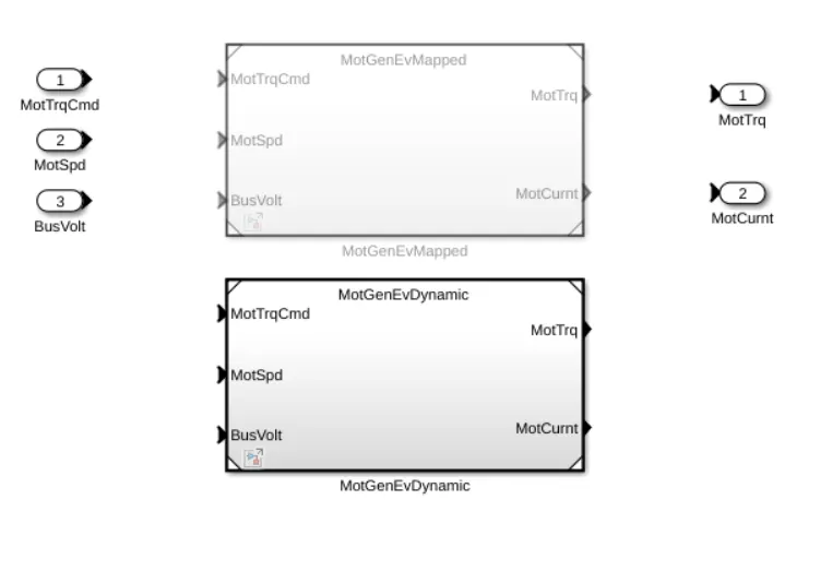
As the same procedure we can do the changing varient from MotGenEVDynamic to MotGenEVMapped for both battery and motor.

This is the changing our model type.

2. How does the model calculate miles per gallon? Which factors are considered to model fuel flow?

Miles per Gallon: Miles per gallon (MPG) is a fuel economy rating determined by how far a car can travel on a gallon of gasoline or deisel. The metric version would be kilometers per litre, MPG is adopted in many metric system countries like canada. While it is both cheaper and better for the environment to achieve a higher MPG rating, there is a curve, that the EPA calls the MPG illusion that shows the cost benefits of increasing MPG decrease with higher rating. Miles per gallon for electric vehicles (MPGe, or “miles per gallon equivalent”) places a value on your car’s energy efficiency. A higher MPGe indicates a higher energy efficiency rating; a lower MPGe indicates a lower rating. Because of this MPG illusion car makers in both the US and Canada are beginning to list there cars. Millege in fuel consumption per distance. In canada this is done in litres per 100 kilometers and in USA this is done in Gallons per 100 Miles (gal/100mi).

But the Focus EV actually requires slightly less than the 33.7 kWh to travel 100 miles (in this case, 32 kWh), so it received an mpg equivalency rating of 105 MPGe. The EPA label provides both city and highway numbers as well as the overall average fuel economy. This mpg-equivalent (MPGe) figure is how the Environmental Protection Agency (EPA) converts the power used by an electric vehicle into a term that's familiar to most Americans: mpg.

The EPA gives each vehicle three different MPG ratings:

1. HIGHWAY MPG: The average a car will get while driving on an open stretch of road without stopping or starting, typically at higher speed.

2. City MPG : The score a car will get an average in city conditions with starting and stopping at lower speeds.

Calculation of miles per gallon in 'EV Reference Application' Model:

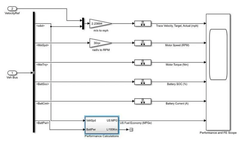
1. Open Ev reference application model in matlab and inside the visualisation block we can see the blocks which are used for calculation of MPG.

2. Now open the performance calculation block.

264.172 US gallons = 1000 L

3. Vehicle speed (x) is multiplied itself and then square rooted. The value is then integrated (1/s) and converted in to meters (m). Then the meters is converted in to miles in the block (m to mile) then it is divided by US gal to get US MPG.

4. For US gallon we need to divide battery power divided by 1000 and thenn divide by 33.7 . Now it is converted from sec to hours by dividing with 3600 then it is converted to m^3 per gal.

5. The values is finally converted into gallon and used as a MPG after dividing miles with gallon.

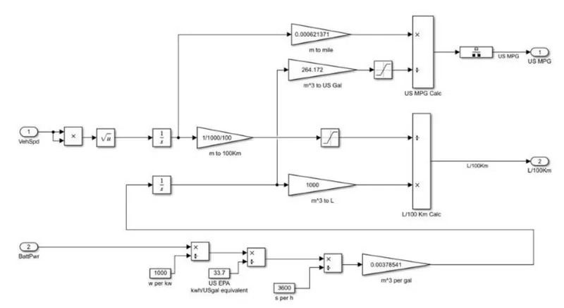
It is multiplied by standard value 0.00378541 to get volume in meters cube per gallon and it is added to the fuel flow forr total value as it is an HEV.

Factors considered in model fuel flow:

1. Vehicle speed

2. Battery power capacity should be high and vehicle power consumption should be low for higher MPGe (Miles Per Gallon Equivalent).

3. Run the HEV ReferenceApplication with WOT drive cycle. Change the grade and wind velocity in the environment block. Comment on the results.

The hybrid electric vehicle reference application represents a full multimode hybrid electric vehicle model with an internal combustion engine, transmission, battery, motor, generator and assosiated powertrain control algorithms. Use the reference application for powertrain matching analysis and component selection control and diagonistic algorithm designe and hardware in the loop (HIL) testing.

By default the HEV multimode reference application is configured with

1. Mapped motor and generator

2. 1.5 L spark plug (SI) dynamic engine.

This diagram shows powertrain configuration:

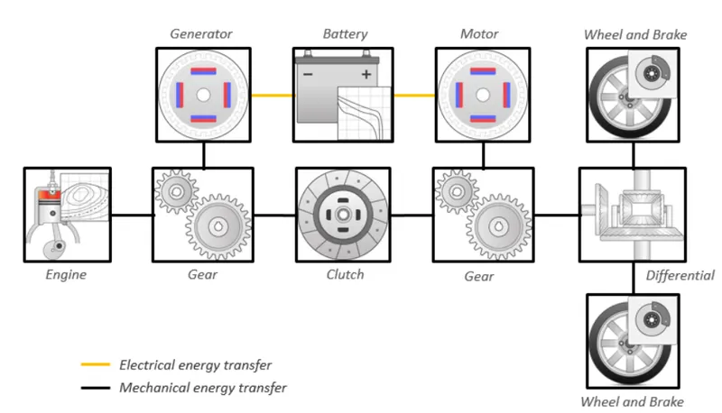
HEV Reference Application Model:

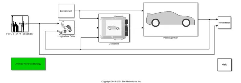
The default drive cycle FTP75 with 2474 sec. Nw change WTO simulation time as 180 sec in the WTO drive cycle.

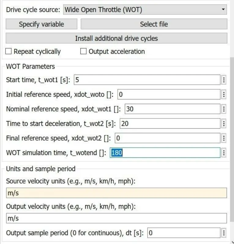
Result:

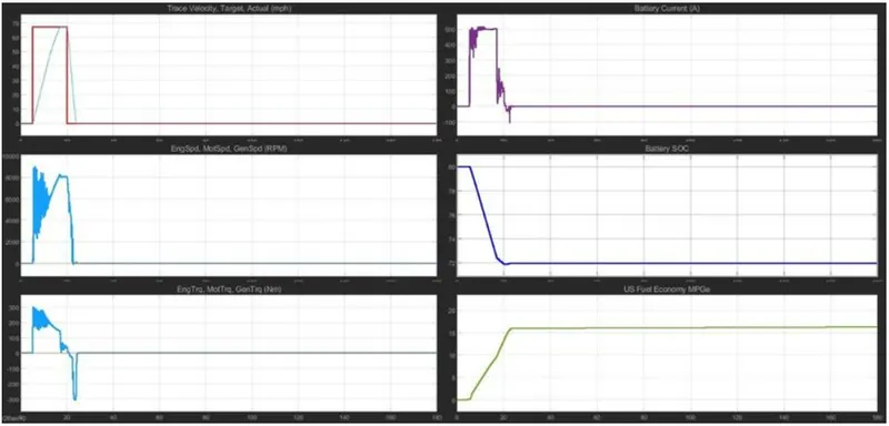
1. The target velocity actual was able to achieve 67.1 mph. The battery current was increased upto 500 Amps in duration of 14 sec.

2.The engine speed is able achieve 8000 RPM and battery state of charge (SOC) was decrease 80 to 71.

GRAPH:

HEV Model with Grade and Wind Velocity:

1. Open the environment subsystem in HEV reference application.

2. Change the grade as 5 and wind velocity as 10.

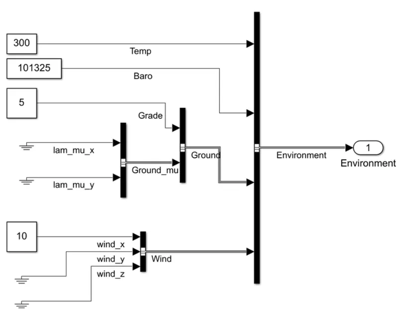
Result:

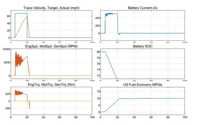
1. We can observe that battery current increased upto 500 and changes occurs upto 20 seconds.

2. At 20 sec the current becomes negative. Battery current is same when compared with above condition.

3. The RPM is positive.

4. The torque is same as previous condition.

5. Due to grade and wind velocity the state of charge (SOC) increase more. It falls below 72 slightly less SOC than previous condition.

4. Keeping all other parameters same, compare the simulated results of hybrid and pure electric powertrains.

HEV Multimode Reference Application:

1. Open HEV reference application model in MATLAB.

2. It consists of drive cycle, environment, longitudinal driver, controller, passenger car and visuals subsystem.

3. Open the environment bolck and change the grade as 5 and wind velocity as 10.

4. Run the simulation with 2474 sec.

Model:

Result:

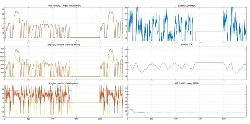
1. First plot shows the drive cycle.

2. Second plot shows the current. It increases and decreases continously throughout the drive cycle.

3. Third plot shows motor speed and engine speed. one speed is almost lower than other time.

4. Fourth plot shows battery SOC. When reaches to 70% the engine produces power and the vehicle is run. It charges for some time upto 80% and continously goes on throughout the drivecycle. During deceleration the battery charges.

5. Fifth plot shows motor torque, engine torque and generator torque.

6. Sixth plot shows fuel economy. Initially it increases up to 28 and maintains almost constant. It decreases and increases around 10. It consists of 250 sec.

EV Referesnce Application:

1. Open EV reference application model in MATLAB.

2. It consists of drive cycle, environment, longitudinal driver, passenger car, and visuals subsystem.

3. Open the environment subsystem and change grade as 5 and wind velocity as 10.

4. Run the simulation with 2474 sec.

Model:

Result:

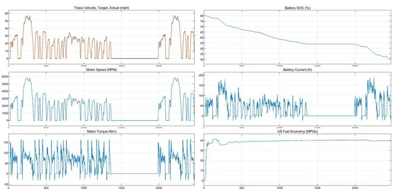
1. First plot shows the drive cycle.

2. Second plot shows the battery SOC. It falls from 80 to 42.

3. Third plot shows motor speed.

4. Fourth plot shows battery current.

5. Fifth plot shows motor torque.

6. Sixth ploth shows fuel economy. Initially it increases 37 to 40. It is almost constant at 40 after 750 sec.