Week 7 State of charge estimation

1.Simulate the 3 test cases from harness dashboard and write a detailed report on the results

2.What is coulomb counting? Refer to the above model and explain how BMS implements coulomb counting for SOC estimation ?

2.Coulomb counting

SOC is a measure of how much charge is available for use in the battery. For the application of rechargeable batteries in H/EVs, SOC is a crucial parameter and thus needs to be measured accurately though electronic and electric systems. It cannot be measured directly because it requires measuring the lithium content at both electrodes. Without accurate SOC measurement, the battery
management system (BMS) would be unable to inform the user when the vehicle needs to be charged or what could be done to improve battery capacity.

A few indirect methods have been discovered to measure the SOC:

Chemical method: applicable only to cells that give open access to their electrolytes (non-sealed lead acid batteries for instance). The SOC can be measured from the specific gravity (hydrometer) or the pH (pH meter) of the electrolyte.

Voltage method: measures the present voltage of the battery to find its SOC using the discharge characteristics of the voltage vs SOC. Not a preferred method because temperature variations are not accounted for in this method which can cause the terminal voltage of a cell to vary from its OCV.

Current integration method (also known as Coulomb counting): involves measuring the amount of current entering and leaving the battery, integrated over time. A device called a coulomb counter will measure the current supplied or removed over a period of time, and will compare it to the pre-programmed capacity of the battery, hence determining the current SOC.

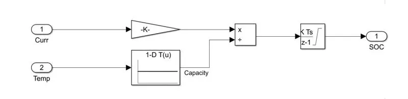
The figure below shows how SOC is modeled. The amount of current entering/leaving the battery is integrated over time and the effect of temperature on capacity is also accounted for by using a 1-D lookup table.

SOC(t) = SOC(t − 1) ⋅ ∫ t t−1 I t ⋅ η Qn ⋅ dt S O C (t) = S O C (t - 1) ⋅ ∫ t - 1 t I

Q = declared/nominal capacity of the cell
n= present efficiency of the cell
i(t)= current flowing in or out

Although this is one of the most common ways of measuring SOC, it still suffers from a lack of reference point. The SOC needs to be recalibrated regularly back to 100% everytime a battery is fully charged, and this is dependent on how accurately the sensor.
determines a fully charged cell. This method also does not consider the changing efficiency of the cell, which is dependent on how much is the charging and discharging current. With greater charge/discharge current, the temperature of the cell increases, which affects efficiency. In addition, over time, the pre-declared capacity (Q) and efficiency of a cell reduces, so reduction in cycle life also affects the SOC measurement.

How BMS implements coulomb counting for SOC estimation in the above mode

BMS implements coulomb couting for SOC estimation in the above, which we can observe in the BMS ECU block. This can be opened by clicking on the BMS_system. The following model will appears if we click on the model.

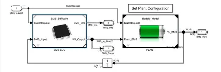
In the above block we can see the subsystem of BMS ECU whic takes the state request and perform the respective operations then gives the information to the Plant of the battery pack. So if we click on the BMS ECU block we can see the following subsystems.

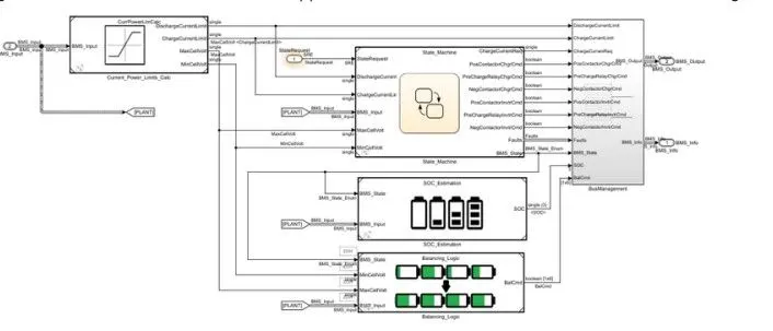
we can see the current power limits subsytem, state machine, SOC estimation, Balancing logic and BMS controller. Here after performing the respective operation the total information will be given to the BMS management where it will further process the data. In the SOC estimation subsystem will perform all the required formulas or methods to calculate the SOC of the vehicle. And will give this to BMS management from there it will gives us the indication.

1.Simulate the 3 test cases from harness dashboard and write a detailed report on the results

first we click and download matlab file and extract into the folder we used the file according to matlab version after that open the file into the matlab and click on system and open the model and open the close loop _ harness dashboard . and run the simulations for 3 differents cases to simulate the results .

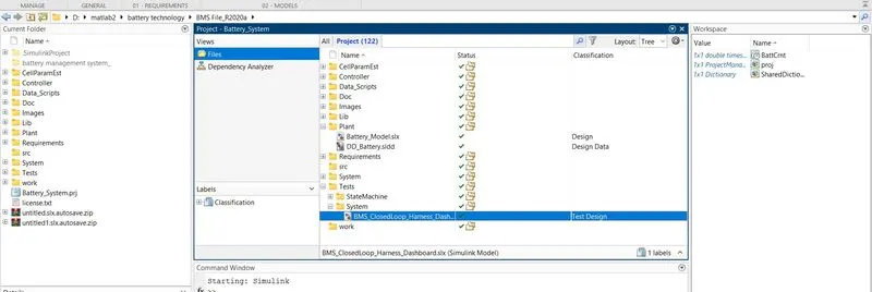
before i selected battery pack 1 so my outputs will be clear mention following things first open BMS system and from projects shortcuts which is top window .

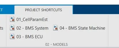
after the selected as BMS_system first click on plant configurations .

Let we simulate the 3 cases and write report on same

case-1 :

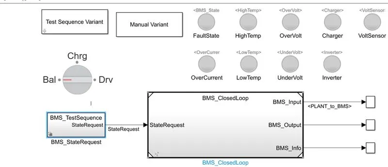
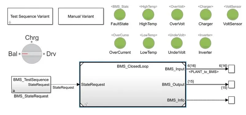
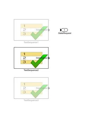
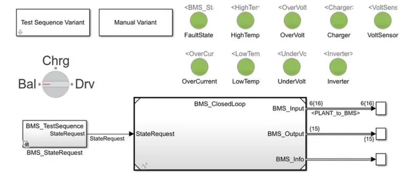
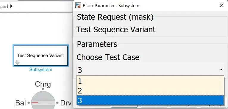
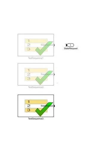
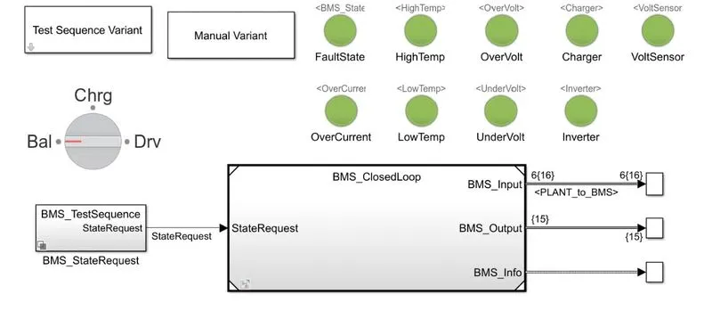
from above figures shown the diffrents subsystems from the test variant subsystem we can selects the test sequece out-off the 3 case which we have to perform test . The manual test variant subsystem shows or used unders the certains situations .

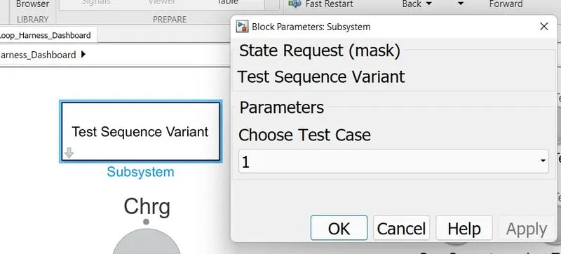
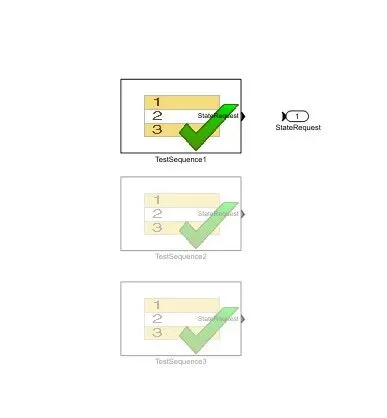
Now we come on the block BMS_ state request it gives which test is to perform let select case 1 . other case 2 will be off .

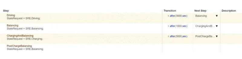
1-Battery is in driving mode for first 3000 secs
2-The next 1000 secs it is cell balancing as the BMS has come to a standby. This will generally only happen when the vehicle hascome to a stop for a long time.
3-The next 5000 seconds are for charging BMS continues to be in standby for the remaining 11,000 seconds

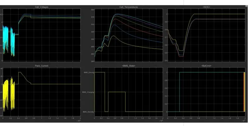
OBSERVATIONS:
1. Fluctuations in cell voltages and pack current until 3000sec indicates that the vehicle was in driving mode
2. Cell voltages start off differently which means there was SOC imbalancing from the beginning. However, they do start converging after 3000sec as cell balancing begins, and by the end of 20,000sec all cells stabilize around 4.1V.
3. Between 4000sec and 9000sec there is constant current (CC) and constant voltage (CV) charging happening: from 4000 - 4600sec it is CC and then the remaining is CV. During CC the SOC increases much more quickly, and then slows down during CV as a precaution mechanism to avoid charging past the voltage limit
4. There is a moderate difference in the temperatures of Cell 1 (297K) and Cell 6 (303K) when the vehicle comes to a stop at 3000sec. This is because of the way the battery pack is assembled. Cell 1 is open to the atmosphere while Cell 6 is thermally insulated on one side. The difference in their peak temperatures is 15 degrees C, and this happens during the initial charging stages. Even at the end of the simulation, when the BMS has been in standby mode for >10000sec the difference in temperature of cell 1 and cell 6 is still 15 degrees C. This really points to the importance of how vital it is to maintain a similar temperature throughout the whole pack, otherwise it will lead to difference between individual cells, such as their voltages, discharge capacities, cycle life or cell degradation, etc.
5. The SOC graph shows the estimation of SOC through different methods, with yellow corresponding to coulomb counting, blue for Unscented Kalman Filter (UKF), and orange for Extended Kalman Filter (EKF). Both Kalman filter methods are evidently more accurate than coulomb counting due to their ability to account for voltage information (the difference between OCV and (sum of voltage drops).

TEST CASE 2

let select case 2 .

.

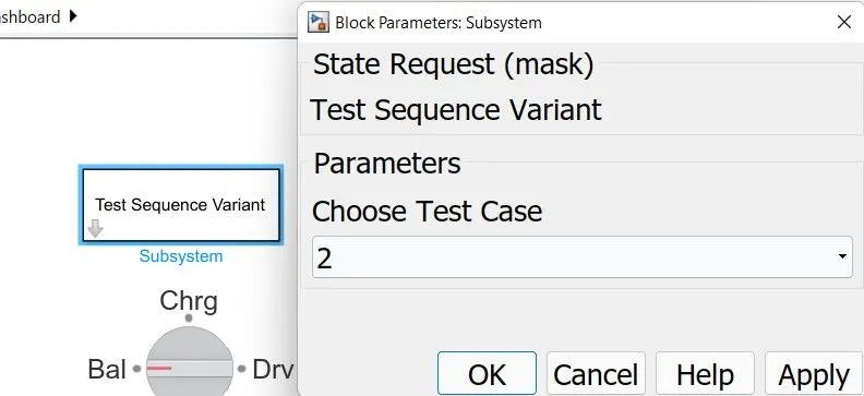
let select case 2 . other case 2 will be off .

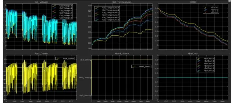
From the above plot, following observations has been identified. Before explaining the plots it should noted that here only 2 modes are happening one is driving mode and then charging mode will activates.

1. From the first plot we can say that is complete driving mode so there is many variations according to the drive cycle. Here the voltage level is varying from 3.2-3.9V intially. But due to the continues driving there is a gradual decrease in the voltage ranges also so we can see that at end the voltage varies between around 3.1-3.7V.

2. In the second plot we can see the temperature of the six cells. As the vehicle is in driving mode, the temperature is continuously increasing due to the high running time.

3. From the SOC plot we can observe that, the SOC is intially at 80%, while driving the SOC is starts discharging, even though there are charge and discharge conditions in the driving mode the running time is high so the SOC is reached to its 0% at 8692seconds. So its not even completed its driving duration also. Which we have set for 10000sec. So all the plot stops at that time because at 0% SOC the vehicle stops then there is no other changes.

4. In the pack current plot, we can see the current variations according to the drive cycle.Intially it is varying between -70A to 15A. But to the long running time the current value also come to around -55A to 20A. And it ends after SOC reaches to 0% as there is no charge to supply.

5. This plot shows the BMS state of operation. As we discussed till now we have only seen the driving mode. So that is why the plot maintains its consistency at Driving mode.

6. In the last plot we can see the Balanced . Since there is no balancing mode it settles at 0 only.

case 3 :

The resultant plot has been observed as shown in the following image.

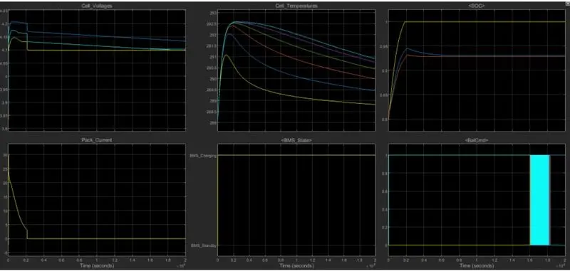
after runnig the simulations select test case3 to getting the folloeing results which are mentions below

1. So from the first plot we can see that, it reaches to full load voltage that is 4.2V and then a small decrease to 4.1V and maintained that value through out the simulation. As this is only charging mode there is no change in the voltage of the cell.
2. From the temperature plot, it can be observed that while battery is in charging condition there is a increment in the temeperature of the cells. But after the battery is full charged the temperature values are quitely settled at normal temperature.
3. In SOC plot we can observe that, it is charged from 80% to 100% in 2000seconds and then it maintains its constant 100% throughout the simulation.
4. From the pack current plot it can be say that, while battery is in charging mode there is a rise in current from 0A to 20A, but after the battery gets fully charged the pack current comes to 0A and then settled.
5. The mode in this case is only charging so the BMS state plot shows only the charging mode.
6. As there is only charging mode, the balancing mode maintains at 1. Which shows in the last plot.