Week 7 State of charge estimation

1.Simulate the 3 test cases from harness dashboard and write a detailed report on the results

Ans

We have to extract the file from the downloaded zip folder,from the battery model,we have to open the BMS system and closed harness dashboard,We can see the closed harness dashboard below,

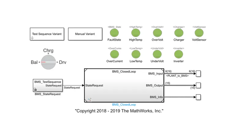
In this model,we can see the Test sequence variant subsystem which consists of 3 different test cases,and the green light indicates the system is working perfectly,and the red light represents  errors in the system.

We have to proceed the 3 test conditions in the BMS test sequence ,for that first we have to choose the test 1 sequence from the Test Sequence Variant subsystem,

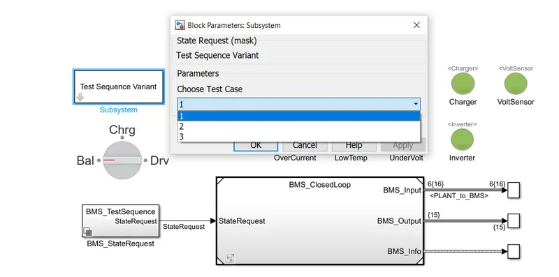
From the BMS_StaeRequest we have to select the testSequence1 

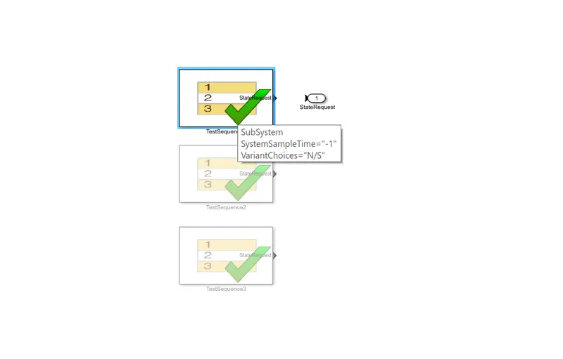
The table below shows the properties of the testsequence1

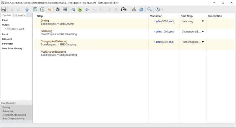
• The first condition is Driving and is set for 3000 seconds
• The second stage is balancing and the duration is 1000seconds
• The third condition is ChargingAndBalancing where it is ran for 5000 seconds
• After that we have post charge balancing till the end of the simulation.

Now we have to simulate the model and examine the results,

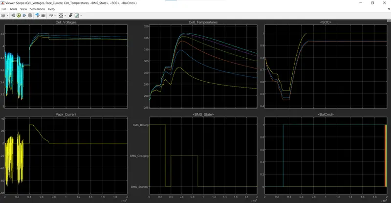
From the Cell Voltage graph we can see the voltage varies form 3.2V to 3.9V according to the driving condition,We can see the variation according to the discharge of the system,after 3000s the voltage goes constantly for the next stage form 3000 to 4000,where the standby occurs for 1000 seconds in the balancing stage,The third condition is charging and balancing,where the voltage graph shows a sudden rise form 3.7V to 4.2V ,and after that we are seeing a slight decrease where it is decreasing to 4.1V,and for post charging condition the voltage is going at a constant rate till the end of the simulation.

From the cell temperature graph the initial temperature is 288K and and gradually all the 6 cell temperature is rising the first cell temperature is rising upto a value of 298K and the 6th cell is reaching at the range of 302K.this is range for the first driving condition,FOr second condition that is balancing we can see the temperature is decreasing for a little range it decreases to 298K for first cell and after 1000s the temperature has got a exponential increase upto a value of 318K for the 6th cell and 302K for the first cell.In the post charge condition we can see the declination of the graph,for the sixth cell it is 308K and for first cell it is around 292K at the end of the simulation.

For SoC graph we have the initial SoC is 80% and in the drive cycle condition it falls to 45% for the 6th cell and 55% for the 1rst cell, And the next conditon is balancing where the graph achieve a standby condition for 1000s and in the next cycle chargig and balancing we can see the sudden rise in the SOC upto a value of 100% and 92% it keeps  the same  value for post charging it goeas constantly till the end of the simulation.

From the pack current graph we can see in the driving condition the current variates from the value of 10A and -70A for the pack and the frequency is also high for 3000s and when it is in second condition,it achieves a standby mode for cell balancing and variation can be seen from 8A to -65A and continues for the next condition a sudden rise can be seen upto a value of 30A and gradually decreases till the end of the stage.In the post charging condition it goes constantly keepiing a zero value.

In the BMS state graph at the driving stage we can see that intially it is in the driving condition for 3000s,In the next stage it is showing the stand by condition of cell balancing for 1000s,and after that achieves charging mode for 5000s and goes standby till the end of the simulation.

In the balancing cells,we can see the cell 6 increases from zero to 1 after the driving stage ,but the cell 1 is showing constant value for all 3 stage conditions and at the post charging mode the cells are reaching the value of one.

Test case 2

we have select the test 2 sequence from the Test Sequence Variant subsystem,

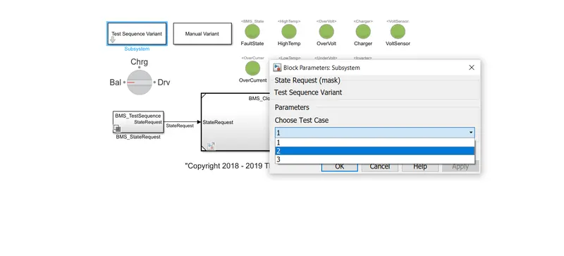
From the BMS_StateRequest we have to select the testSequence2

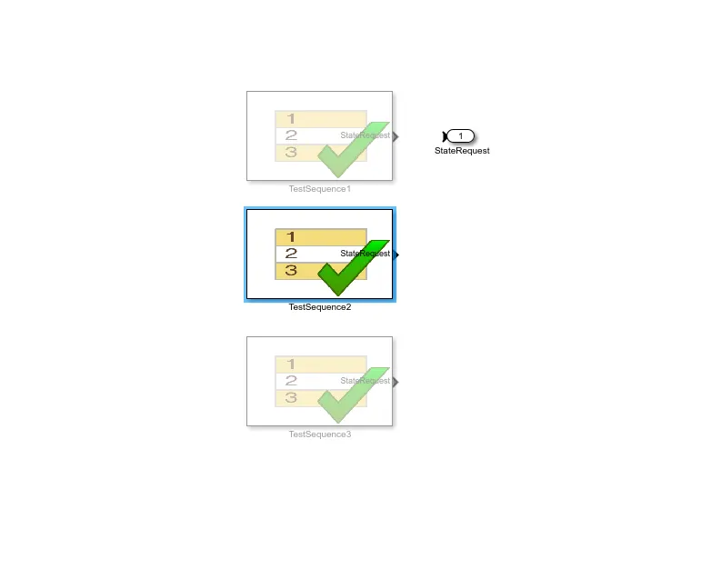
The table below shows the properties of the testsequence2

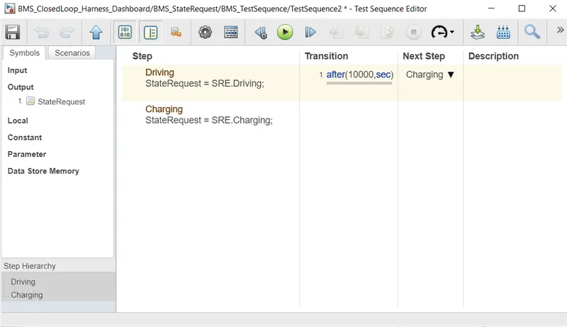
From the test properties,the test sequence consist of 2 stages,Driving and charging ,the simulation is done for 20000 seconds. We can examine the results,

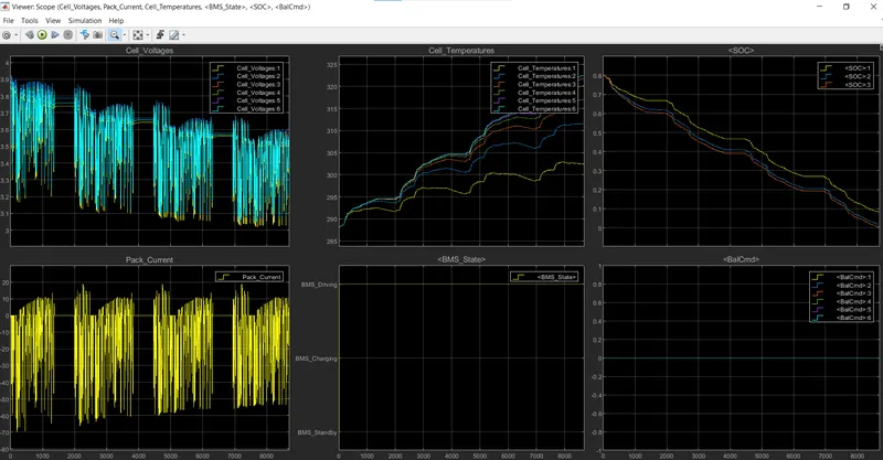
From the cell voltage graph we can see that up to 9000 seconds, the cell voltages range from maximum 3.9V to 3.05V as cutoff voltage.between the variation we can see  some areas it shows some linearity, At 9000 seconds, the entire capacity was depleted.

In the cell temperature graph we can see the temperature rise from 288K to 322K ,Cell 1 has a lower temperature variation, ranging from 288K to around 302.5K.Cell 6 has a higher temperature range, ranging from 288K to around 322.5K.As these durations are in standby modes, the cell temperatures are slightly lowering in between the drive modes.

We can see the variation in the SOC graph,the initial condition is 80% and gradually decreases with respect to the time.In the full drive mode, as seen in the above plot, the SOC drops from 80% to 0% (as current is drained for a longer period of time). The SOC remains constant in standby states in between them.The first cell is not reaching the value of zero at the end of the simulation time.

In the pack current graph,the current variates from the value of 10A and -70A for the pack and the frequency is also high,During the overall drive, the pack current discharges up to 70A and little charging occurs.In between the drive modes, there are some standby mode conditions.

In the BMS state graph the graph is showing only that it is operating in the driving mode.The graph changes from standby mode to driving mode for rest of the simulation time.

In the cell  balancing graph it is showing zero value through out the simulation.

Test case 3-

For simulating the third case We have to select the test 3 sequence from the Test Sequence Variant subsystem,

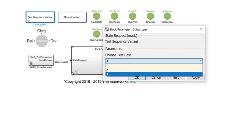
From the BMS_StateRequest block we have to select the testSequence3

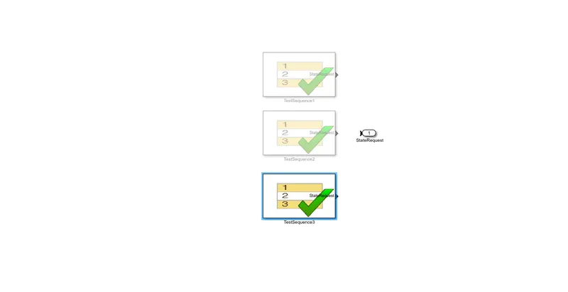
The table below shows the properties of the testsequence3

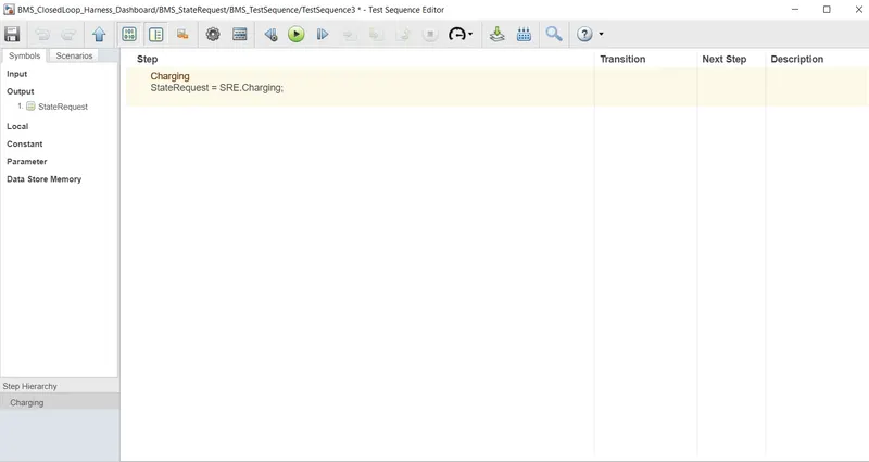
In this case we have only one stage that is charging for the complete simulation time.We can see the plots below,

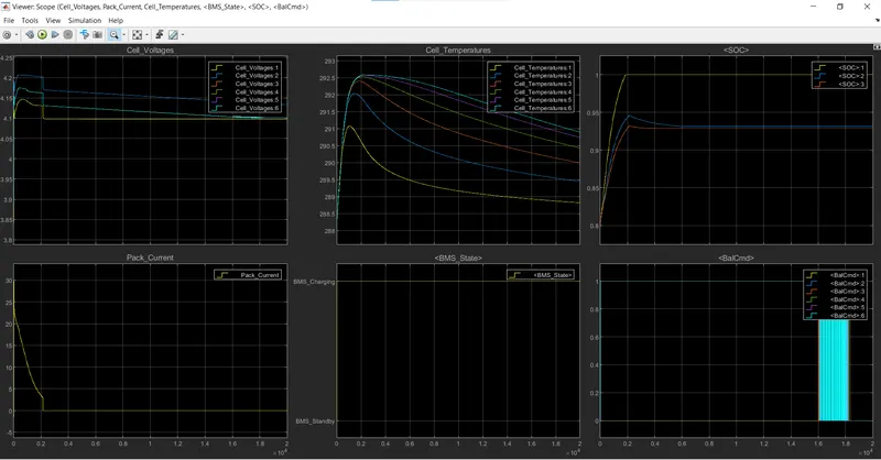
From the cell voltage graph we can see that Initially, the voltage in cell 2 climbs from 3.9V to 4.2V  before stabilising at 4.15V. After 2000 seconds we can see the graph goes linearly downlwards till the end of the simulation.Cell 1 goes from 3.85V to 4.1V and then settles at 4.08V.

In the cell temperature graph,intially there is a sudden rise in the temperature of the cells,it goes from 288K to 292.5K and the decreases exponentially till the end of the simulation.

In the SOC graph we can see the increase in the range of the SOC,from 80% to 100% the cell 1 becomes the highest of the value and the ceel 2 and 3 reaches the value of 92.5% and accomodes in that value till the end of the simulation.

In pack current graph,we can see the sudden declination from 30 to 0 . The graph reaches zero in the 2000s and goes constant until the end of the simulation.

In the BMS state we can see the graph is going in the charging state and in balancing cell graph,the cell 1 is balancing in the simulation time. 

2.What is coulomb counting? Refer to the above model and explain how BMS implements coulomb counting for SOC estimation ? 

Ans-Coulomb counting is a technique for tracking a battery pack's State of Charge. It calculates the overall sum of energy entering or exiting the battery pack by integrating the active flowing current (measured in amps) over time. This results in a capacity that is usually expressed in Amp-hours,

When a battery is fully charged, SOC (State Of Charge) is defined as the ratio of available capacity to maximum capacity, and it reflects the remaining percentage of the battery capacity. The coulomb counting method is used to calculate the SOC percent.
To estimate SOC, the coulomb counting method analyses the battery's discharging current and integrates the discharging current over time. Which can be calculated using the discharging current (I(t)) and previously calculated SOC values (SOC(t-1)). The relationship can be expressed as follows,

`SOC=SOC(t-1)frac{I(t)}{underset(n)(Q)} trianglet`

In modified coulomb counting the discharge current is corrected with a function and corrected current is used for SOC calculation,we can write the equation as,

`underset(c)(I)(t)=underset(2)(K)I(t)^2+underset(1)(K)I(t)+underset(0)(K)`

And SOC equation can be written as,

`SOC(t)=SOC(t-1)+ frac{underset(c)(I)(t)}{underset(n)(Q)}trianglet`

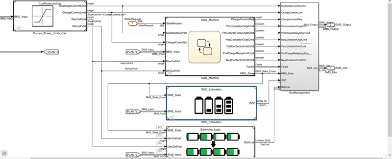
We have the Coulomb counting technique in the BMS model,so we look into the SOC estimation subsystem,

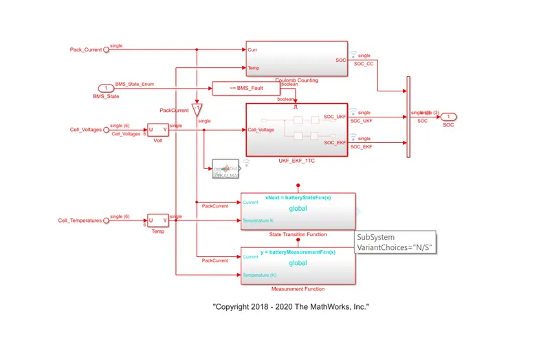
In the coulomb counting susbsytem,we have the configuration as shown below,

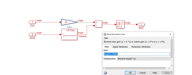
To convert current to Ahr, the discharge current from the battery is given to gain with a value of 1/3600.Temperature changes cause the value to be split by capacity.

Then, because we're using a discrete integrator, we'll integrate with a gain of 1 and a sample time of -1.

Saturation thresholds range from 0 to 1.We'll multiply the SOC values from 0 to 1 by 100 to get a percentage of SOC.