Week 7 - Simulation of a 1D Supersonic nozzle flow simulation using Macormack Method
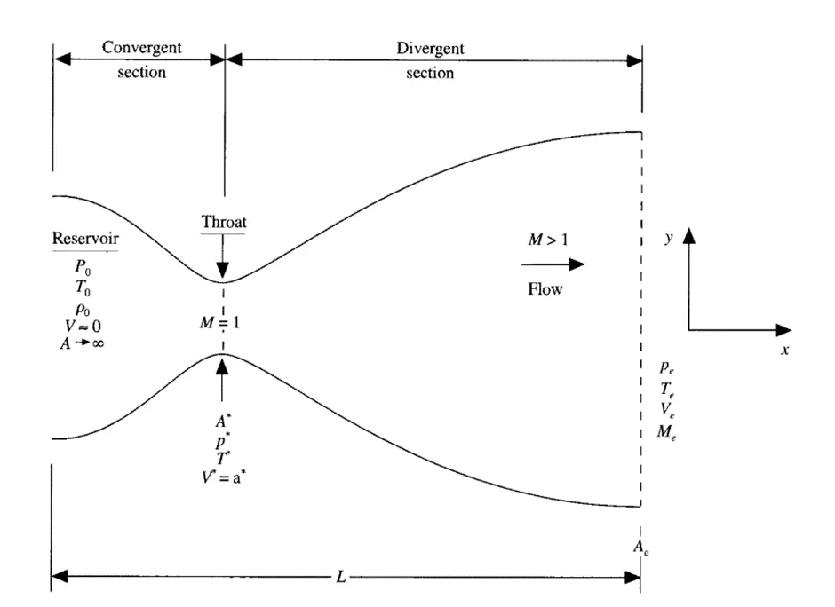
Description of the Problem:Steady isoentropic flow through a convergent-divergent nozzle is considered. The flow at the inlet originates from a reservoir where the values of pressure, temperature and density are denoted by 'P0', 'T0','`rho`0'. The cross-sectional area of the reservoir is assumed to be large enough for the inlet velocity to attain a negligible value.Thus, 'P0' and 'T0' are stagnation values (or total temperatures and pressures respectively).The flow expands isoentropically towards the exit. The exit pressure, temperature, velocity and mach number are represented as 'Pe', 'Te', 'Ve' and 'Me' respectively. The flow is locally subsonic at the convergent section, sonic at the throat section and super-sonic at the divergent section. The values of the flow variables at the throat section (sonic flow values as the mach number here is '1') is denoted by with an accompanying asterisk ('∗').
We make an assumption that at a given section that across any elemental cross section, the flow properties are uniform. This implies that the flow variables only vary with 'x'. Thus, the problem is reduced to a 1D problem. Since, this is not truly a 1D problem, a more accurate term would be 'Quasi 1-Dimensional'.
Governing Equations:
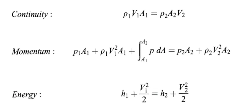
Non-Condervative form:
Continuity:
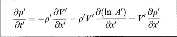
Momentum conservation:
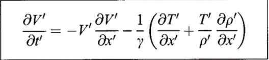
Energy Conseervation:

Conservative form:(in terms of solution vectors ('U'), flux vectors ('F') and source terms ('J'))
(Where 1,2,3 denotes the vectors associated with continuity, momentum conservation and energy conservation equations respectively.)
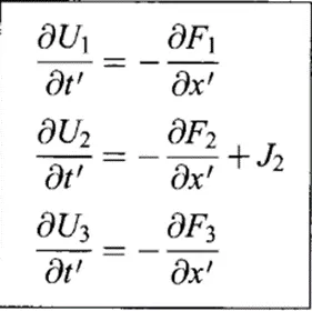
where,
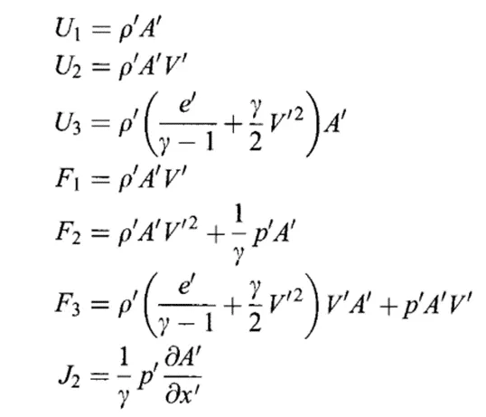
Conservative and non-conservative forms of these governing differential equations are mathematically equivalent.
Now, we move on to discretising these equations. Finite Difference McCormack's Explicit Method is a predictor/corrector method that is second order accurate in both space and time.
First is the predictor step, where the spatial variables are set-up in the forward-differencing scheme to find the predicted time-derivative.



We then obtain, the predicted values of '`rho`','V','T'.
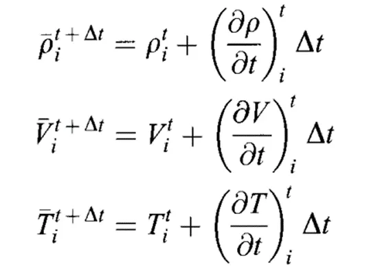
We then move to the corrector step where the only difference is that the forward differencing scheme in the spatial derivatives is replaced by backward differencing and the updated values are used.
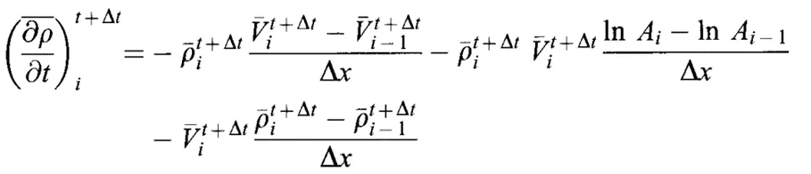

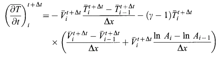
The avverage time-derivates are thus calculated:
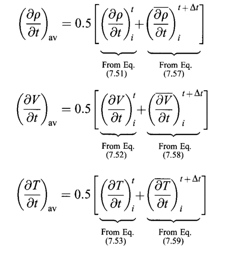
These "averaged" time-derivatives are used in calculating the final values of the flow-field variables at the end of the time-step.
The same approach is used for discretising the conservational form too.
For calculating the time-step:
The following formula is used to locally calculate the time step for each grid point. Here, 'a' denotes the local velocity of sound and 'V' is the local flow velocity.
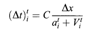
The least value of these calculated time-steps is what is used for all calculations.
The initial and boundary conditions are referenced from the prescribed textbook.
Main Code:
close all
clear
clc
%defining the 1-D mesh:
L=3; n=31; x=linspace(0,3,n); dx=x(2)-x(1); nt=1400;gamma=1.4;R=8.3145;
%Initial Profiles:
rho=1-0.3146*x; rho_i=rho;
T=1-0.2314*x; T_i=T;
v=(0.1+1.09*x).*T.*0.5; v_i=v;
a=1+2.2*(x-1.5).^2;
a_s=(gamma*R*T).^(1/2);
rho_old=rho;
v_old=v;
T_old=T;
for i=1:n
    if x(i)<=0.5
        rho_p(i)=1;
        T_p(i)=1;
    elseif x(i)>=0.5 && x(i)<=1.5
        rho_p(i)=1-0.366*(x(i)-0.5);
        T_p(i)=1-0.167*(x(i)-0.5);
    elseif x(i)>=1.5 && x(i)<=3.5
        rho_p(i)=0.634-0.3879*(x(i)-1.5);
        T_p(i)=0.833-0.3507*(x(i)-1.5);
    end
end
v_p=0.59*(rho_p.*a).^(-1);
%Incorporating the CFL criteria:
C=0.85;
del_t=((a_s+v).^-1)*dx*0.8;
dt=min(del_t);
%Calling the functions:
[rho_nc2, v_nc2, T_nc2,mfr_nc2,rho_th_nc2,v_th_nc2,T_th_nc2]=non_cons2(rho,v,T,a,x,nt,dt,n);
[rho_c, v_c, T_c,mfr_c,rho_th_c,v_th_c,T_th_c]=cons(rho_p,v_p,T_p,a,x,nt,dt,n);
%Plotting the steady state distribution of primitive variables:
subplot(3,1,1)
plot(x,rho_nc2,'--',x,rho_c,':')
title('Density along the nozzle')
xlabel('x')
ylabel('Density')
legend('Non-conservative','Conservative')
subplot(3,1,2)
plot(x,v_nc2,'--',x,v_c,':')
title('Velocity along the nozzle')
xlabel('x')
ylabel('Velocity')
legend('Non-conservative','Conservative')
subplot(3,1,3)
plot(x,T_nc2,'--',x,T_c,':')
title('Temperature along the nozzle')
xlabel('x')
ylabel('Temperature')
legend('Non-conservative','Conservative')
%Plotting the time-stepwise variation of primitive variables:
tstep=1:1400;
figure(2)
subplot(3,1,1)
plot(tstep,rho_th_nc2,'--',tstep,rho_th_c,':')
xlabel('Time-Step')
ylabel('Throat Density')
title('Throat Density vs Time-Step')
legend('Non-conservative','Conservative')
subplot(3,1,2)
plot(tstep,v_th_nc2,'--',tstep,v_th_c,':')
xlabel('Time-Step')
ylabel('Throat Velocity')
title('Throat Velocity vs Time-Step')
legend('Non-conservative','Conservative')
subplot(3,1,3)
plot(tstep,T_th_nc2,'--',tstep,T_th_c,':')
xlabel('Time-Step')
ylabel('Throat Temperature')
title('Throat Temperature vs Time-Step')
legend('Non-conservative','Conservative')
%Plotting the mass flow rate at the throats vs time-step:
figure(3)
plot(tstep,mfr_nc2,'--',tstep,mfr_c,':')
title('Mass Flow Rate at Different Time-Steps')
xlabel('Time-Step')
ylabel('MFR at the Throat')
legend('Non-conservative','Conservative')
figure(4)
mfr_c_ss=rho_c.*a.*v_c;
mfr_nc2_ss=rho_nc2.*a.*v_nc2;
plot(x,mfr_nc2_ss,'--',x,mfr_c_ss,':')
title('Mass Flow Rate along the Nozzle')
xlabel('x')
ylabel('Normalised Mass Flow Rate')
Function for the solution of the Non-Conservative form:
function [rho,v,T,mfr,rho_th,v_th,T_th]=non_cons2(rho,v,T,a,x,nt,dt,n)
dx=x(2)-x(1);
gamma=1.4;

for k=1:nt
rho_old=rho;
v_old=v;
T_old=T;
%rho_i=rho;
%v_i=v;
%T_i=T;
for i=2:n-1
%Predictor Step:
dvdx(i)=(v(i+1)-v(i))/(dx);
dlnadx(i)=(log(a(i+1))-log(a(i)))/(dx);
drhodx(i)=(rho(i+1)-rho(i))/(dx);
dTdx(i)=(T(i+1)-T(i))/(dx);

drhodt_p(i)=-rho(i)*dvdx(i)-rho(i)*v(i)*dlnadx(i)-v(i)*drhodx(i);
dvdt_p(i)=-v(i)*dvdx(i)-(1/gamma)*(dTdx(i)+(T(i)/rho(i))*drhodx(i));
dTdt_p(i)=-v(i)*dTdx(i)-(gamma-1)*T(i)*(dvdx(i)+v(i)*dlnadx(i));

%Updating the values:
rho(i)=rho_old(i)+drhodt_p(i)*dt;
v(i)=v_old(i)+dvdt_p(i)*dt;
T(i)=T_old(i)+dTdt_p(i)*dt;
end

for i=2:n-1
%Corrector step (using the updated values):
dvdx(i)=(v(i)-v(i-1))/(dx);
dlnadx(i)=(log(a(i))-log(a(i-1)))/(dx);
drhodx(i)=(rho(i)-rho(i-1))/(dx);
dTdx(i)=(T(i)-T(i-1))/(dx);

drhodt_c(i)=-rho(i)*dvdx(i)-rho(i)*v(i)*dlnadx(i)-v(i)*drhodx(i);
dvdt_c(i)=-v(i)*dvdx(i)-(1/gamma)*(dTdx(i)+(T(i)/rho(i))*drhodx(i));
dTdx_c(i)=-v(i)*dTdx(i)-(gamma-1)*T(i)*(dvdx(i)+v(i)*dlnadx(i));
end

%Average Time Derivative that will be used for the final values of the
%time-step;
drhodt_av=(drhodt_p+drhodt_c)/2;
dvdt_av=(dvdt_p+dvdt_c)/2;
dTdt_av=(dTdt_p+dTdx_c);

%Final Values:
for i=2:n-1
rho(i)=rho_old(i)+drhodt_av(i)*dt;
v(i)=v_old(i)+dvdt_av(i)*dt;
T(i)=T_old(i)+dTdt_av(i)*dt;
end

%Boundary Conditions:
v(1) = 2*v(2)-v(3);

v(n) = 2*v(n-1)-v(n-2);
rho(n) = 2*rho(n-1)-rho(n-2);
T(n) = 2*T(n-1)-T(n-2);
%Mass flow rate:
mfr(k)=rho(16)*a(16)*v(16);
v_th(k)=v(16);
rho_th(k)=rho(16);
T_th(k)=T(16);
end

end
Function for the solution of the Conservative form:
function [rho,v,T,mfr,rho_th,v_th,T_th]=cons(rho,v,T,a,x,nt,dt,n)
dx=x(2)-x(1);
rho_old=rho;
v_old=v;
T_old=T;
gamma=1.4;
%Solution vectors:
u1=rho.*a; u2=rho.*a.*v; u3=rho.*(T/(gamma-1)+(gamma/2)*v.^2).*a;
for k=1:nt
%Flux vectors:
f1=rho.*a.*v; f2=rho.*a.*v.^2+(1/gamma)*rho.*T.*a;
f3=rho.*(T/(gamma-1)+(gamma/2)*v.^2).*a.*v+rho.*T.*a.*v;
%Source Terms:
for l=2:n-1
    dadx(l)=(a(l+1)-a(l))/dx;
    j2(l)=(1/gamma)*rho(l)*T(l)*dadx(l);
end

u1_i=u1; u2_i=u2; u3_i=u3;
for i=2:n-1
%Predictor Step:
du1dt_p(i)=-(f1(i+1)-f1(i))/dx;
du2dt_p(i)=-(f2(i+1)-f2(i))/(dx)+j2(i);
du3dt_p(i)=-(f3(i+1)-f3(i))/dx;
%Updating the values:
u1(i)=u1(i)+du1dt_p(i)*dt;
u2(i)=u2(i)+du2dt_p(i)*dt;
u3(i)=u3(i)+du3dt_p(i)*dt;
end

%Updating rho,v,T:
rho=u1./a; v=u2./u1; T=(gamma-1)*(u3./u1-(gamma/2)*v.^2);
%Flux vectors:
f1=rho.*a.*v; f2=rho.*a.*v.^2+(1/gamma)*rho.*T.*a;
f3=rho.*(T/(gamma-1)+(gamma/2)*v.^2).*a.*v+rho.*T.*a.*v;
%Source Terms:
for l=2:n-1
    dadx(l)=(a(l)-a(l-1))/dx;
    j2(l)=(1/gamma)*rho(l)*T(l)*dadx(l);
end

%Predictor Step, averaged derivative and updating the final values:
for i=2:n-1
du1dt_c(i)=-(f1(i)-f1(i-1))/dx;
du2dt_c(i)=-(f2(i)-f2(i-1))/(dx)+j2(i);
du3dt_c(i)=-(f3(i)-f3(i-1))/dx;

du1dt_av(i)=(du1dt_p(i)+du1dt_c(i))/2;
du2dt_av(i)=(du2dt_p(i)+du2dt_c(i))/2;
du3dt_av(i)=(du3dt_p(i)+du3dt_c(i))/2;

u1(i)=u1_i(i)+du1dt_av(i)*dt;
u2(i)=u2_i(i)+du2dt_av(i)*dt;
u3(i)=u3_i(i)+du3dt_av(i)*dt;
end
%Boundary Conditions:
u1(1)=rho(1)*a(1);
u2(1)=2*u2(2)-u2(3);
u3(1)=u1(1)*(T(1)/(gamma-1)+gamma/(2)*v(1)^2);

u1(n)=2*(u1(n-1))-(u1(n-2));
u2(n)=2*(u2(n-1))-(u2(n-2));
u3(n)=2*(u3(n-1))-(u3(n-2));
%Evaluating the primitive variables:
rho=u1./a; v=u2./u1; T=(gamma-1)*(u3./u1-(gamma/2)*v.^2);
mfr(k)=rho(16)*a(16)*v(16);
v_th(k)=v(16);
rho_th(k)=rho(16);
T_th(k)=T(16);
end
end
Obtained Results:
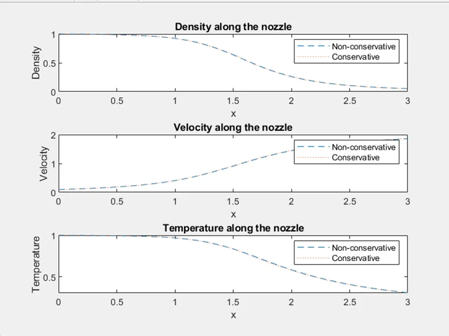
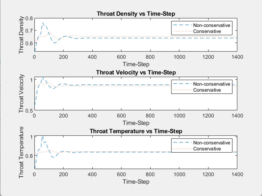
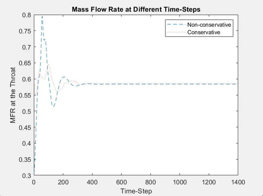
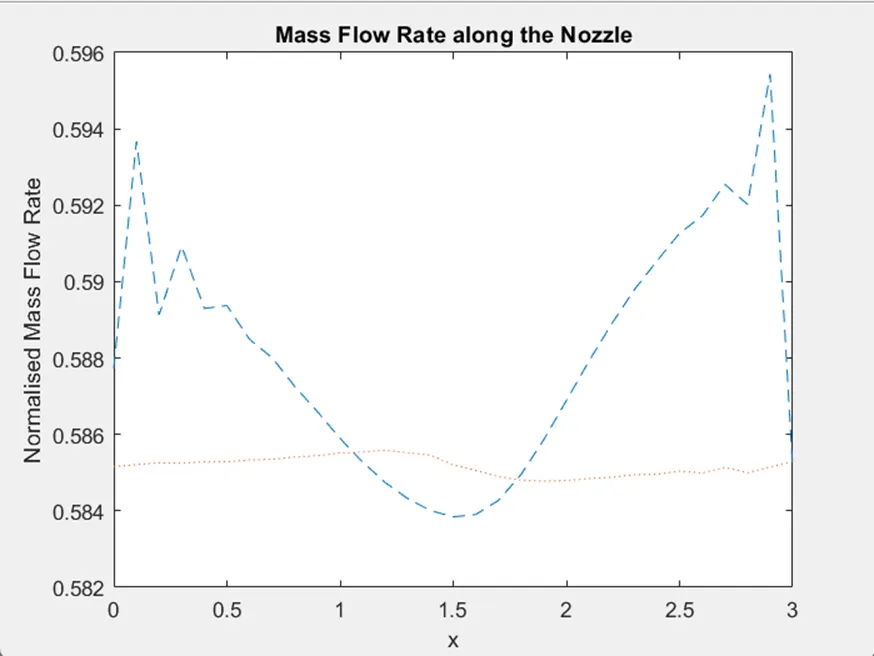
To perform a grid independance test, the entire code was run with 'n(=number of nodes)=101' (a much finer mesh):
Revised main code with 'n=101':
close all
clear
clc
%defining the 1-D mesh:
L=3; n=101; x=linspace(0,3,n); dx=x(2)-x(1); nt=1400;gamma=1.4;R=8.3145;
%Initial Profiles:
rho=1-0.3146*x; rho_i=rho;
T=1-0.2314*x; T_i=T;
v=(0.1+1.09*x).*T.*0.5; v_i=v;
a=1+2.2*(x-1.5).^2;
a_s=(gamma*R*T).^(1/2);
rho_old=rho;
v_old=v;
T_old=T;
for i=1:n
    if x(i)<=0.5
        rho_p(i)=1;
        T_p(i)=1;
    elseif x(i)>=0.5 && x(i)<=1.5
        rho_p(i)=1-0.366*(x(i)-0.5);
        T_p(i)=1-0.167*(x(i)-0.5);
    elseif x(i)>=1.5 && x(i)<=3.5
        rho_p(i)=0.634-0.3879*(x(i)-1.5);
        T_p(i)=0.833-0.3507*(x(i)-1.5);
    end
end
v_p=0.59*(rho_p.*a).^(-1);
%Incorporating the CFL criteria:
C=0.85;
del_t=((a_s+v).^-1)*dx*0.8;
dt=min(del_t);
%Calling the functions:
[rho_nc2, v_nc2, T_nc2,mfr_nc2,rho_th_nc2,v_th_nc2,T_th_nc2]=non_cons2(rho,v,T,a,x,nt,dt,n);
[rho_c, v_c, T_c,mfr_c,rho_th_c,v_th_c,T_th_c]=cons(rho_p,v_p,T_p,a,x,nt,dt,n);
%Plotting the steady state distribution of primitive variables:
subplot(3,1,1)
plot(x,rho_nc2,'--',x,rho_c,':')
title('Density along the nozzle')
xlabel('x')
ylabel('Density')
legend('Non-conservative','Conservative')
subplot(3,1,2)
plot(x,v_nc2,'--',x,v_c,':')
title('Velocity along the nozzle')
xlabel('x')
ylabel('Velocity')
legend('Non-conservative','Conservative')
subplot(3,1,3)
plot(x,T_nc2,'--',x,T_c,':')
title('Temperature along the nozzle')
xlabel('x')
ylabel('Temperature')
legend('Non-conservative','Conservative')
%Plotting the time-stepwise variation of primitive variables:
tstep=1:1400;
figure(2)
subplot(3,1,1)
plot(tstep,rho_th_nc2,'--',tstep,rho_th_c,':')
xlabel('Time-Step')
ylabel('Throat Density')
title('Throat Density vs Time-Step')
legend('Non-conservative','Conservative')
subplot(3,1,2)
plot(tstep,v_th_nc2,'--',tstep,v_th_c,':')
xlabel('Time-Step')
ylabel('Throat Velocity')
title('Throat Velocity vs Time-Step')
legend('Non-conservative','Conservative')
subplot(3,1,3)
plot(tstep,T_th_nc2,'--',tstep,T_th_c,':')
xlabel('Time-Step')
ylabel('Throat Temperature')
title('Throat Temperature vs Time-Step')
legend('Non-conservative','Conservative')
%Plotting the mass flow rate at the throats vs time-step:
figure(3)
plot(tstep,mfr_nc2,'--',tstep,mfr_c,':')
title('Mass Flow Rate at Different Time-Steps')
xlabel('Time-Step')
ylabel('MFR at the Throat')
legend('Non-conservative','Conservative')
figure(4)
mfr_c_ss=rho_c.*a.*v_c;
mfr_nc2_ss=rho_nc2.*a.*v_nc2;
plot(x,mfr_nc2_ss,'--',x,mfr_c_ss,':')
title('Mass Flow Rate along the Nozzle')
xlabel('x')
ylabel('Normalised Mass Flow Rate')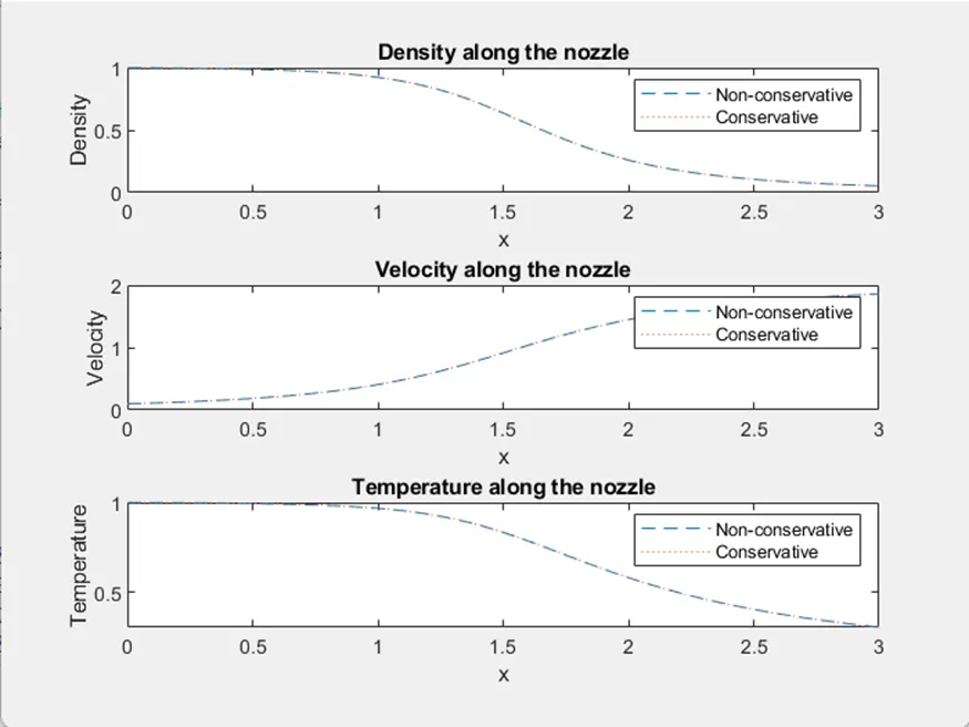
(The obtained steady state plots are similar. This affirms grid indepemdance).
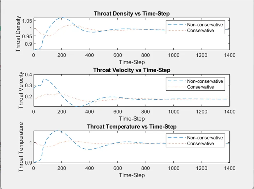
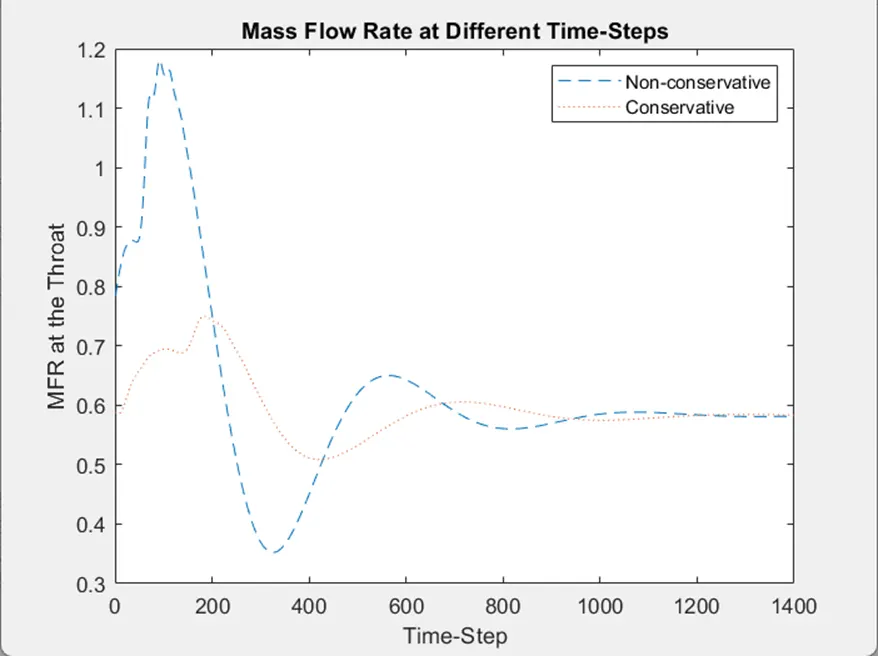
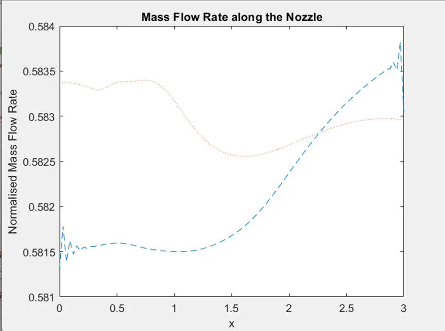
(The normalised mass flow rate is fluctuating lesser in comparison to the coarser mesh.)
Conclusions and findings:
This project investigates a compressible, steady, isentropic flow through convergent-divergent nozzle. The physics modelled in the code is massively simplified by assuming that the flow field variables change only with 'x' (thereby making it quasi 1 Dimensional).
The problem has been modelled by numerically solving both the Conservative and Non-Conservative forms of the governing equations that have been discretised by McCormack's method.
Despite being mathematically equivalent, on numerically solving both these forms, the obtained graphs for the mass flow rates at steady state show small variations.
The graphs showing the variables changing with the time-steps are also slightly different for the conservative and non conservative forms.
However the steady state distributions for the flow field variables (density, velocity and temperature) obtained from both forms are the same.
Increasing the mesh fineness increases the accuracy of the results but imposes a higher computational cost.