Week 7 - Simulation of a 1D Supersonic nozzle flow simulation using Macormack Method

Introduction

The study focuses on simulating isentropic flow through a quasi 1D convergent divergent nozzle. Both conservation and non conservation forms of the governing equations are derived and solved using the MacCormack's technique. The primary objective include determining the steady stste temperature distribution, comparing solutions from both forms and analysing mass flow rate distributions.

Methodology

Governing Equations

The governing equations for isentropic flow include the continuity, momentum and energy equations. Thses are expressed in both conservation and non conserbation forms.

Non-Conservative Form

Continuity Equation

`(delrho)/(delt)+u(delrho)/(delx)+rho(delu)/(delx)+rhou 1/A (dA)/(dx) = 0`

Momentum Equation

`(delu)/(delt)+u(delu)/(delx) + 1/rho (delrho)/(delx) = 0`

Energy Equation (for isentropic flow, pressure and density are related via `p=p^(gamma)`)

`(delT)/(delt) + u(delT)/(delx) + (gamma-1)T((delu)/(delx)+u 1/A (dA)/(dx)) = 0`

Conservative Form

Conservation of Mass

`(del(rhoA))/(delt) + (del(rhouA))/(delx) = 0`

Conservation of Momentum

`(del(rhouA))/(delt) + (del(rhou^2A+pA))/(delx) = p(dA)/(dx)`

Conservation of Energy

`(del(rhoEA))/(delt) + (del[(rhoE+p)uA])/(delx) = 0`

Where:

• `rho` is the density
• `u` is the velocity
• `p` is the pressure
• `A` is the area
• `E = p/((gamma-1)rho) = (u^2)/2` is the total energy per unit mass
• `gamma` is the specific heat ratio

MacCormack's Technique

The MacCormack's method is a second order accurate, two step predictor corrector scheme used to solve the above equation in time, Its is paricularly suited for hyperbolic PDEs and is applied here for both conservative and non conservative forms.

• Predictor Step (Forward Difference):
  Estimates the variables at the next time level using a forward spatial derivative.

• Corector Step (Backward Difference)
  Refines the prediction using a backward spatial derivative and averages it with the predictor result.

This method helps in capturing smooth solutions and shocks with reasonable accuracy.

Initial and Boundary Condition

Initial Condition:

• A uniform distribution of flow variables (pressure, temperature, velocity and density) is assumed throughout the nozzle at `t=0`.

Boundary Conditions:

• Inlet `(x=0)`: Total pressure and temperature are specified.
• Outlet `(x=L)`: Static pressure is prescribed.
• Boundary values are held constant during the simulation to drive the flow development inside the nozzle.

Result and Discussion

Mass Flow Rate Variation (Conservative Form)

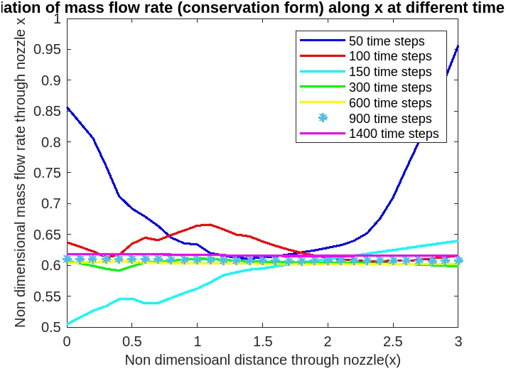
This plot shows how the non dimentional mass flow rate varies along the nozzle length at different time steps using the conservative formulation of MacCormack's method.

At early time steps (50-150), the mass flow rate is highly non uniform, especially near the inlet and outlet, indicating the solution is still transient.

From 300 to 600 time steps, the flow begins to stabilize and the mass flow rate becomes more uniform.

At 900 and 1400 time steps, the mass flow rate is nearly constant across the nozzle, showing that the solution has converged to steady state.

This confirms that the conservative form preserves mass flow accurately and the simulation is numerically stable and physyically consistent.

Mass Flow Rate Variation (Non-Conservative Form)

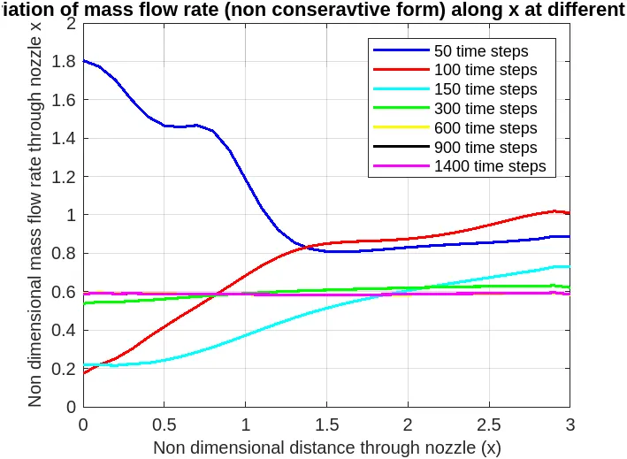
This plot shows the non-dimentional mass flow rate variation along the nozzle using the non-conservative form of MacCormack's methos.

At early time steps (50-150), the masss flow rate is highly inconsistent and shows large deviations from expected values, especially near the inlet.

As the time progress, the solution begins to stabilize, but even at 300 and 600 time steps, the mass flow rate does not remain constant aceoss the nozzle.

Even at 900 and 1400 time steps, although some uniformity is achieved, small deviations persist, indicating the solution is less accurate that the conservative case.

This highlight that the non conservative form does not strictly conserve mass, lading to physical inaccuracies, especially in compressible flow with strong gradients.

Comparison of Mass Flow Rate (Conservative vs Non-Conservative Forms)

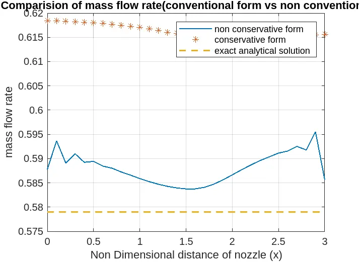
This plot compares the masss flow rate along the nozzle for non conservative form, conservative form and exact analytical solution.

The conservative form stay very close to the exact solution, maintaining a nearly constant mass flow rate across the domain.

The non conservative form shows clear fluctuations and deviation from the exact value, indicating mass conservation is not properly enforced.

The conservative method is thus more accurate and physically reliable, especially for problem involving compressible flow through varying cross section.

Mach Number Profile (Conservative vs Non-Conservative)

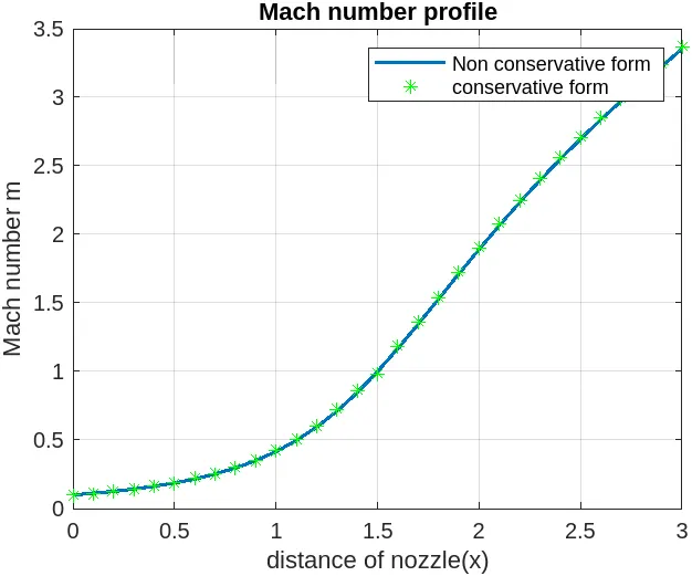
This plot compares the Mach number distribution along the nozzle for both conservative and non conservative forms.

Both methods show excellent agreement in the Mach number profile.

The flow accelerates smoothly from subsonic `(M<1)` to supersonic `(M>1)`, with the sonic point `(M=1)` near the throat of the nozzle.

Despite the mass conservation issue in the non conservative form, it still captures the Mach number accurately, likely due to its strong dependence on the mementum and energy equations.

Both methods predict the velocity fields (Mach number) accurately, bit only the conservative form ensures proper mass conservation.

Temperature Change (Conservative vs Non-Conservative Form)

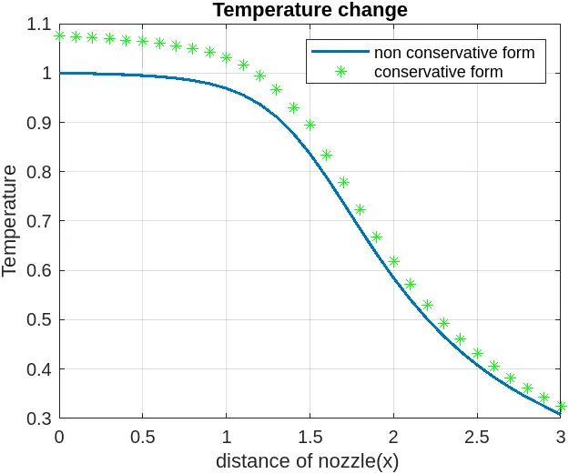
This plot compares the temperature variation along the nozzle for both forms.

Temperature decrease steadily along the nozzle due to isentropic expansion.

The conservation form consistently predicts higher temperature than the non conservative form.

Both methods follow the same overall trend, but there is a noticeable deviation especially in the diverging section.

While both methods capture the cooling trend, the conservative form is more physically accurate, particularly in high speed (supersonic) regions.

Pressure Change (Conservative vs Non-Conservative Form)

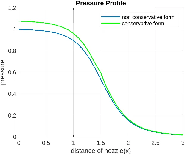
This plot compares the pressure variation along the nozzle for both forms.

In the convergent section, the conservative form predicts slightly higher pressure than the non conservative form, indicating better accuracy near the throat.

As the flow enters the diverging section, both profiles begin to converge, showing good agreement in the supersonic region where area changes have less influence on discrepancies between the two methods.

Velocity Change (Conservative vs Non-Conservative Form)

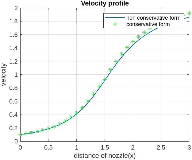
This plot compares the temperature variation along the nozzle for both forms.

In the convergent section, both the conservative and non conservative forms show good agreement, with velocity increasing smoothly.

Beyond the throat, in the diverging section, the conservative form slightly over predicts the velocity compared to the non conservative form, but the difference gradually decreases as the flow progress.

This indicate that the conservative form maintains better accuracy in capturing rapid acceleration in supersonic flow.

Density Change (Conservative vs Non-Conservative Form)

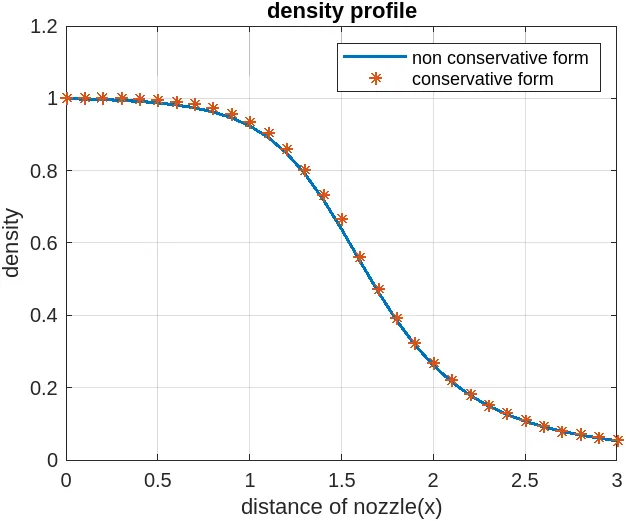
This plot compares the density variation along the nozzle for both forms.

The density decreases steadily along the nozzle, reflecting acceleration of the flow. Both conservative and non conservative forms match closely throughout the domain.

Slight deviations occur near the throat and in the diverging section, but the difference is minimal.

This suggests that both formulations are equally reliable for capturing density variations in quasi 1D isentropic nozzle flow.

Temperature Change vs Time Steps(Conservative vs Non-Conservative Form)

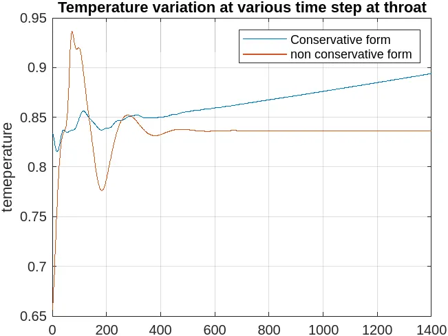
The non conservative form reaches a steady state faster with minimal long term variation, indicating quicker numerical convergence.

The conservative form, however shows a gradual increase in temperature over time, hinting at slower convergence or possible accumulation of numerical errors.

Both forms exhibit early stage oscillations, but the non conservative form stabilizes more quickly.

While the non conservative foem is numerically more stable at the throat,the conservative form may require finer control on time step or flux handling to achieve steady results.

Pressure Change vs Time Steps(Conservative vs Non-Conservative Form)

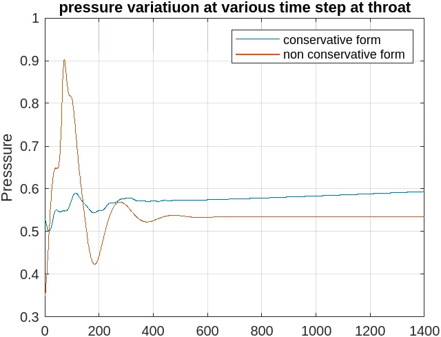
The non conservative form stabilizes earlier, showing a nearly flat behavior after approximately 500 time steps.

The conservative form continues to rise gradually, suggesting slower convergence and possible residual numerical dissipation.

Initial transient oscillations are present in both forms, but they damp out faster in the non conservative form.

The non conservatice form shows faster and smoother convergence for pressure at the throat, while the conservative form demands more iterations to reach a steady value.

Density Change vs Time Steps(Conservative vs Non-Conservative Form)

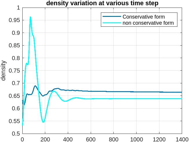
The non conservative form shows stronger initial oscillations and overshoots, but settles to a steady value faster, around 500 steps.

The conservative form exhibits smoother but slower convergence, with a gradual approach to steady state.

Final steady values of both forms are close, but the paths to convergence differ significantly.

The non convergence form converges faster but is more prone to initial instability, while the conservative form is more stable over time, though slower to reach steady density.

Conclusion

This study analyzed the quasi 1D isentropic nozzle flow using MacCormack's method in both conservative and non conservative forms, focusing on the evolution and steady state behavior of velocity, pressure, density and temperature.

The conservative formulation is more numerically robust, particularly in maintaining physical consistency and suppressing spurious oscillations.

The non conservative formulation is computationally efficient and converges faster, but mau suffer form stability issues, especially under sharge gradient conditions.

Final Verdict

For accurate and stable simulation, the conservatconservative form is recommended , especially in the floes invloving shocks or high gradient zones. The non conservative form can be suitable for faster convergence in simpler or well behaved problems but demands careful time step and stability considerations.