Week 7 - Simulation of a 1D Supersonic nozzle flow simulation using Macormack Method
Aim: Simulation of a 1D Supersonic nozzle flow simulation using Macormack Method using MATLAB.
Objective:
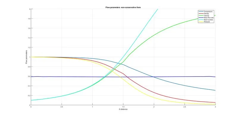
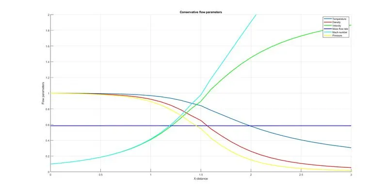
- Steady-state distribution of primitive variables inside the nozzle
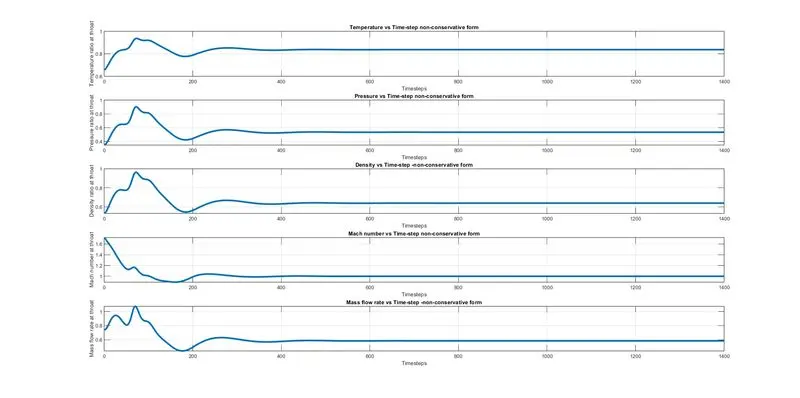
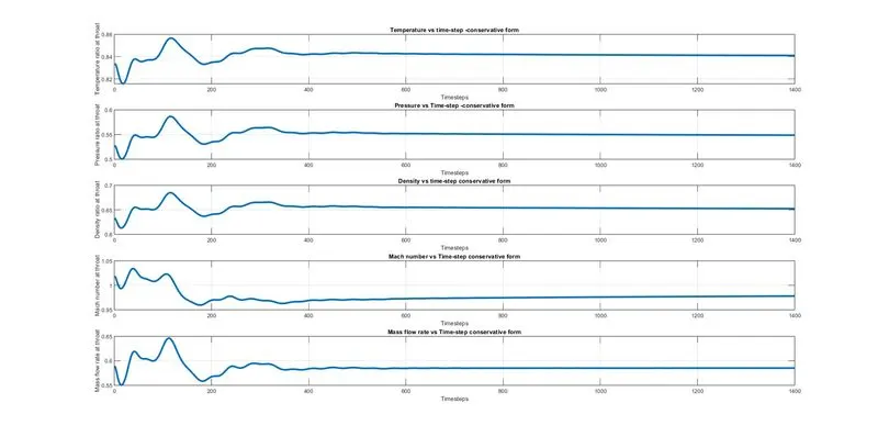
- Time-wise variation of the primitive variables.
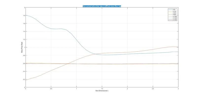
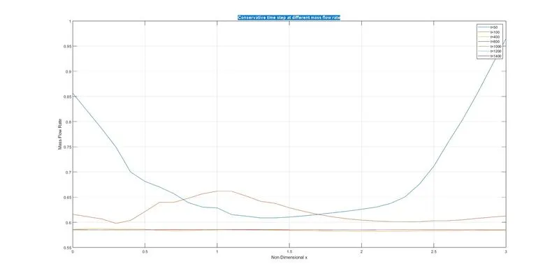
- Variation of Mass flow rate distribution inside the nozzle at different time steps during the time-marching process.
- Comparison of Normalized mass flow rate distributions of both forms.
- Perform a grid independence test on the solution and explain all your findings.
- The code must be modular. You need to write separate functions to solve both forms.
- Discuss all the plots you are providing with observed inferences.
Theory:
To simulate a 1D supersonic nozzle flow using the MacCormack method in MATLAB, we'll need to implement the MacCormack algorithm within a loop to solve the Euler equations for compressible flow. The Euler equations for 1D compressible flow are:
To simulate the isentropic flow through a quasi-1D subsonic-supersonic nozzle, we'll start by deriving both the conservation and non-conservation forms of the governing equations. Then, we'll use the MacCormack's technique to solve these equations and determine the steady-state temperature distribution for the flow-field variables. Finally, we'll compare the solutions obtained using the two forms of the governing equations to investigate their differences.
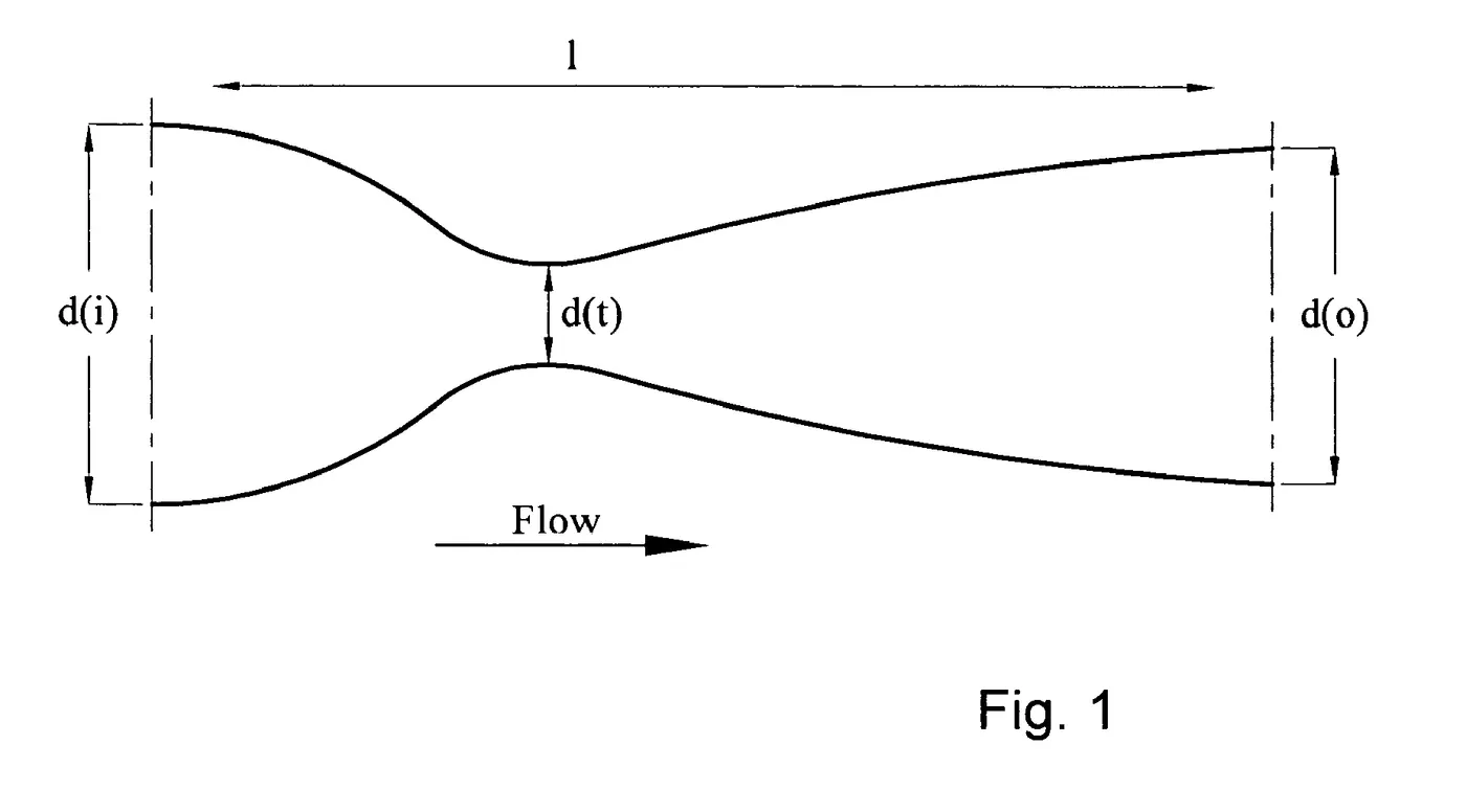
Let's first derive the governing equations:
- Conservation Form: The conservative form of the Euler equations for 1D steady, compressible flow through a nozzle are:
- Continuity Equation:
`(∂(ρA))/(∂x) = 0` - Momentum Equation:
`(∂(ρuA))/(∂x) + (∂(PA))/(∂x) = 0` - Energy Equation:
`(∂(ρhA))/(∂x) + (∂(uhA))/(∂x) + (∂(qA))/(∂x) = 0`
where:=,- `ρ` is the density
- `u` is the velocity
- `A` is the cross-sectional area of the nozzle
- `P` is the pressure
- `h` is the enthalpy
- `q` is the heat flux
- Continuity Equation:
- Non-Conservation Form: The non-conservative form of the Euler equations for the same flow are:
- Continuity Equation:
∂ρ/∂x + ρ(1/A)∂A/∂x = 0 - Momentum Equation:
∂(ρu)/∂x + ∂(u^2 + P/ρ)/∂x - u/A ∂A/∂x = 0 - Energy Equation:
∂(ρh)/∂x + ∂(uh)/∂x + P(1/A)∂A/∂x - q/A = 0
where, `h` is the specific enthalpy.
- Continuity Equation:
Now, let's implement the MacCormack's technique to solve both the conservative and non-conservative forms of these equations to obtain the steady-state temperature distribution and compare their solutions.
MacCormack's Technique:
The MacCormack's method is a finite difference-based numerical technique used for time-accurate solutions of partial differential equations. It is an explicit two-step predictor-corrector method, which is particularly useful for solving hyperbolic conservation laws.
In MacCormack's method, the governing equations are first discretized in space and time using finite differences. Then, a predictor step and a corrector step are performed at each time step.
-
Predictor Step: Using the conservative or non-conservative form of the equations, we calculate the predicted values at the next time step based on the current values.
-
Corrector Step: We calculate the corrector values by taking the average of the predictor values and the original values. This helps to improve the stability and accuracy of the method.
The predictor and corrector steps are repeated until the solution converges to the steady-state. The convergence is checked based on a predefined tolerance level.
By applying MacCormack's method to both the conservative and non-conservative forms of the governing equations, we can obtain the steady-state temperature distribution and compare the solutions obtained from these two forms.
MATLAB Code :
- Function code for Conservative from:
function[mdot_throat,rho_throat,M_throat,T_throat,P_throat,t,M,P,rho,v,mdot]=conservative(n,x,dx,throat,a,cfl) %inputs n = 31; x = linspace(0,3,n); dx = x(2)-x(1); throat = (n+1)/2; cfl = 0.5; a = 1+2.2*(x-1.5).^2; for i = 1:n if x(i)>=0 && x(i)<=0.5 rho(i) = 1; t(i) = 1; elseif x(i)>=0.5 && x(i)<=1.5 rho(i) = 1-0.366*(x(i)-0.5); t(i) = 1-0.167*(x(i)-0.5); elseif x(i)>=1.5 && x(i)<=3.5 rho(i)=0.634-0.3879*(x(i)-1.5); t(i)=0.833-0.3507*(x(i)-1.5); end end v=0.59./(rho.*a); gamma=1.4; %adaptive time step method for d = 1:n A = sqrt(t(d)); dt_i(d) = cfl*(dx/(v(d)+A)); end dt=min(dt_i); nt=1400; %solution vectors u_1 = rho.*a; u_2 = u_1.*v; u_3 = u_1.*((t./(gamma-1))+((gamma/2)*v.^2)); %macormack method for k = 1:nt %predictor step term_1 = (u_2.^2./u_1); term_2 = ((gamma-1)/gamma)*(u_3-(gamma/2)*term_1); term_3 = (gamma*u_2.*u_3)./u_1; term_4 = 0.5*gamma*(gamma-1)*u_2.^3./u_1.^2; F_1 = u_2; F_2 = term_1+term_2; F_3 = term_3-term_4; %creating a copy of the solution vectors u_1_old = u_1; u_2_old = u_2; u_3_old = u_3; for j=2:n-1 %differencing in spatial terms dF_1_dx(j) = (F_1(j+1)-F_1(j))/dx; dF_2_dx(j) = (F_2(j+1)-F_2(j))/dx; dF_3_dx(j) = (F_3(j+1)-F_3(j))/dx; %forward differencing dA_dx=((a(j+1))-(a(j)))/dx; J_2=(1/gamma).*rho(j).*t(j).*dA_dx; %continuity equation du_1_dt_p(j) = -dF_1_dx(j); %momentum equation du_2_dt_p(j) = -dF_2_dx(j)+J_2; %energy equation du_3_dt_p(j) = -dF_3_dx(j); %first solution update u_1(j) = u_1_old(j)+du_1_dt_p(j)*dt; u_2(j) = u_2_old(j)+du_2_dt_p(j)*dt; u_3(j) = u_3_old(j)+du_3_dt_p(j)*dt; end %corrected step term_1 = (u_2.^2./u_1); term_2 = ((gamma-1)/gamma)*(u_3-(gamma/2)*term_1); term_3 = (gamma*u_2.*u_3)./u_1; term_4 = 0.5*gamma*(gamma-1)*u_2.^3./u_1.^2; F_1 = u_2; F_2 = term_1+term_2; F_3 = term_3-term_4; rho = u_1./a; v = u_2./u_1; t = (gamma-1)*((u_3./u_1)-(0.5*gamma*v.^2)); for j = 2:n-1 %backward differencing in spatial terms dF_1_dx(j) = (F_1(j)-F_1(j-1))/dx; dF_2_dx(j) = (F_2(j)-F_2(j-1))/dx; dF_3_dx(j) = (F_3(j)-F_3(j-1))/dx; %backward differencing dA_dx = ((a(j))-(a(j-1)))/dx; J_2 = (1/gamma).*rho(j).*t(j).*dA_dx; %continuity equation du_1_dt_c(j) = -dF_1_dx(j); %momentum equation du_2_dt_c(j) = -dF_2_dx(j)+J_2; %energy equation du_3_dt_c(j) =-dF_3_dx(j); end %computing average du_1_dt_avg=0.5*(du_1_dt_p+du_1_dt_c); du_2_dt_avg=0.5*(du_2_dt_p+du_2_dt_c); du_3_dt_avg=0.5*(du_3_dt_p+du_3_dt_c); %final solution update for j=2:n-1 u_1(j)=u_1_old(j)+du_1_dt_avg(j)*dt; u_2(j)=u_2_old(j)+du_2_dt_avg(j)*dt; u_3(j)=u_3_old(j)+du_3_dt_avg(j)*dt; end %boundary condition u_1(1) = rho(1).*a(1); u_2(1) = 2*u_2(2)-u_2(3); u_3(1) = u_1(1)*((t(1)/(gamma-1)+0.5*gamma*v(1).^2)); %supersonic outflow-point n u_1(n) = 2*u_1(n-1)-u_1(n-2); u_2(n) = 2*u_2(n-1)-u_2(n-2); u_3(n) = 2*u_3(n-1)-u_3(n-2); %solution vectors rho = u_1./a; v = u_2./u_1; t = (gamma-1)*((u_3./u_1)-(0.5*gamma*v.^2)); P = rho.*t; M = v./sqrt(t); mdot = rho.*a.*v; %taking values at throat v_throat(k) = v(throat); rho_throat(k) = rho(throat); T_throat(k) = t(throat); P_throat(k) = P(throat); M_throat(k) = M(throat); mdot_throat(k) = mdot(throat); if k == 50 figure(2) plot(x,mdot) hold on elseif k == 100 figure(2) plot(x,mdot) hold on elseif k == 400 figure(2) plot(x,mdot) hold on elseif k == 800 figure(2) plot(x,mdot) hold on elseif k == 1000 figure(2) plot(x,mdot) hold on elseif k == 1200 figure(2) plot(x,mdot) hold on elseif k == 1400 figure(2) plot(x,mdot) xlabel('Non Dimensional x') ylabel('Mass Flow Rate') legend('t=50','t=100','t=400','t=800','t=1000','t=1200','t=1400'); title('Conservative time step at different mass flow rate') grid on hold on end end - Function code for Non-Conservative from:
function [mdot_throat_nc,rho_throat_nc,M_throat_nc,T_throat_nc,P_throat_nc,t,M_nc,P_nc,rho,v,mdot_nc]=non_conservative(n,x,dx,throat,a,cfl); %inputs n = 31; x = linspace(0,3,n); dx = x(2)-x(1); throat = (n+1)/2; a = 1+2.2*(x-1.5).^2; cfl = 0.5; t = 1-0.2314*x; v = (0.1+1.09*x).*t.^0.5; rho = 1-0.3146*x; gamma = 1.4; %calculating the time step for d = 1:n A = sqrt(t(d)); dt_i(d) = cfl*(dx/(v(d)+A)); end dt = min(dt_i); nt = 1400; %NON-CONSERVATIVE FORM for k = 1:nt rho_old = rho; v_old = v; T_old = t; %predicted step-forward differencing for i = 2:n-1 %defining spatial terms dv_dx = (v(i+1)-v(i))/dx; drho_dx = (rho(i+1)-rho(i))/dx; dlog_A_dx = (log(a(i+1))-log(a(i)))/dx; dt_dx = (t(i+1)-t(i))/dx; %continuity equation drho_dt_p(i) = -rho(i)*dv_dx-rho(i)*v(i)*dlog_A_dx-v(i)*drho_dx; %momentum equation dv_dt_p(i) = -v(i)*dv_dx-(1/gamma)*(dt_dx+(t(i)/rho(i))*drho_dx); %energy equation dT_dt_p(i) = -v(i)*dt_dx-(gamma-1)*t(i)*(dv_dx+v(i)*dlog_A_dx); %first solution update rho(i) = rho_old(i)+drho_dt_p(i)*dt; v(i) = v_old(i)+dv_dt_p(i)*dt; t(i) = T_old(i)+dT_dt_p(i)*dt; end %corrected step for i = 2:n-1 %defining spatial terms dv_dx = (v(i)-v(i-1))/dx; dlog_A_dx = (log(a(i))-log(a(i-1)))/dx; drho_dx = (rho(i)-rho(i-1))/dx; dt_dx = (t(i)-t(i-1))/dx; %continuity equation drho_dt_c(i) = -rho(i)*dv_dx-rho(i)*v(i)*dlog_A_dx-v(i)*drho_dx; %momentum equation dv_dt_c(i) = -v(i)*dv_dx-(1/gamma)*(dt_dx+(t(i)/rho(i))*drho_dx); %energy equation dT_dt_c(i) = -v(i)*dt_dx-(gamma-1)*t(i)*(dv_dx+v(i)*dlog_A_dx); end %average time derivative drho_dt_avg = 0.5*(drho_dt_p+drho_dt_c); dv_dt_avg = 0.5*(dv_dt_p+dv_dt_c); dT_dt_avg = 0.5*(dT_dt_p+dT_dt_c); %final solution update for i = 2:n-1 v(i) = v_old(i)+dv_dt_avg(i)*dt; t(i) = T_old(i)+dT_dt_avg(i)*dt; rho(i) = rho_old(i)+drho_dt_avg(i)*dt; end %inlet update v(1) = 2*v(2)-v(3); rho(1) = 1; t(1) = 1; %outlet update v(n) = 2*v(n-1)-v(n-2); rho(n) = 2*rho(n-1)-rho(n-2); t(n) = 2*t(n-1)-t(n-2); %finding primitive variables mdot_nc = rho.*a.*v; M_nc = v./sqrt(t); P_nc = rho.*t; %throat value v_throat_nc(k) = v(throat); rho_throat_nc(k) = rho(throat); T_throat_nc(k) = t(throat); P_throat_nc(k) = P_nc(throat); M_throat_nc(k) = M_nc(throat); mdot_throat_nc(k) = mdot_nc(throat); if k == 50 figure(1) plot(x,mdot_nc) hold on elseif k == 100 figure(1) plot(x,mdot_nc) hold on elseif k == 400 figure(1) plot(x,mdot_nc) hold on elseif k == 800 figure(1) plot(x,mdot_nc) hold on elseif k == 1000 figure(1) plot(x,mdot_nc) hold on elseif k == 1200 figure(1) plot(x,mdot_nc) hold on elseif k == 1400 figure(1) plot(x,mdot_nc) xlabel('Non Dimensional x') ylabel('Mass Flow Rate') legend('t=50','t=100','t=400','t=800','t=1000','t=1200','t=1400'); title('Non-conservative time step at diffrent mass flow rate') grid on hold on end end - Main code:
clear all close all clc n=31; x=linspace(0,3,n); dx=x(2)-x(1); cfl=0.5; throat=(n+1)/2; a=1+2.2*(x-1.5).^2; %Initial profile %Non Conservative [mdot_throat_nc,rho_throat_nc,M_throat_nc,T_throat_nc,P_throat_nc,t,M_nc,P_nc,rho,v,mdot_nc]=non_conservative(n,x,dx,throat,a,cfl); %Conservative [mdot_throat,rho_throat,M_throat,T_throat,P_throat,t,M,P,rho,v,mdot]=conservative(n,x,dx,throat,a,cfl); %COMPARISON GRAPHS figure(3) hold on plot(x,mdot) plot(x,mdot_nc) ylim([0.575 0.62]) set(gca,'YTick',(0.575:0.005:0.62)) xlabel('X') ylabel('Mass flow rate') grid on legend('Conservative','Non-conservative') title('Mass flow rate conservative vs non-conservative') figure(4) subplot(4,1,1) hold on plot(M_throat,'linewidth',3) plot(M_throat_nc,'linewidth',3) xlabel('Timesteps') ylabel('Mach number') legend('Conservative','Non-conservative') title('Mach number variation at throat for conservative and non-conservative') subplot(4,1,2) hold on plot(T_throat,'linewidth',3) plot(T_throat_nc,'linewidth',3) xlabel('Timesteps') ylabel('Temperature') legend('Conservative','Non-conservative') title('Temperature variation at throat for conservative and non-conservative') subplot(4,1,3) hold on plot(P_throat,'linewidth',3) plot(P_throat_nc,'linewidth',3) xlabel('Timesteps') ylabel('Pressure') legend('Conservative','Non-conservative') title('Pressure variation at throat for conservative and non-conservative') subplot(4,1,4) hold on plot(rho_throat,'linewidth',3) plot(rho_throat_nc,'linewidth',3) xlabel('timesteps') ylabel('Density') legend('Conservative','Non-conservative') title('Density variation at throat for conservative and non-conservative') %Non conservative form figure(5) subplot(4,1,1) plot(x,t) axis([0 3.1 0 1.1]) xlabel('X-distance') ylabel('Temperature ratio') title('Flow parameters non-conservative form') subplot(4,1,2) plot(x,M_nc) xlabel('x-distance') ylabel('mach number') subplot(4,1,3) plot(x,P_nc) xlabel('X-distance') ylabel('Pressure ratio') subplot(4,1,4) plot(x,rho) xlabel('X-distance') ylabel('Density ratio') figure(6) hold on plot(x,t,'linewidth',2) plot(x,rho,'linewidth',2,'color','r') plot(x,v,'linewidth',2,'color','g') plot(x,mdot_nc,'linewidth',2,'color','b') plot(x,M_nc,'linewidth',2,'color','c') plot(x,P_nc,'linewidth',2,'color','y') xlabel('X-distance') ylabel('Flow parameters') grid on legend('Temperature','Density','Velocity','Mass flow rate','Mach number','Pressure') title('Flow parameters -non-conservative form') ylim([0 2]) set(gca,'YTick',(0:0.2:2)) figure(7) subplot(5,1,1) plot(T_throat_nc,'linewidth',3) xlabel('Timesteps') ylabel('Temperature ratio at throat') grid on title('Temperature vs Time-step non-conservative form') subplot(5,1,2) plot(P_throat_nc,'linewidth',3) xlabel('Timesteps') ylabel('Pressure ratio at throat') grid on title('Pressure vs Time-step non-conservative form') subplot(5,1,3) plot(rho_throat_nc,'linewidth',3) xlabel('Timesteps') ylabel('Density ratio at throat') grid on title('Density vs Time-step -non-conservative form') subplot(5,1,4) plot(M_throat_nc,'linewidth',3) xlabel('Timesteps') ylabel('Mach number at throat') grid on title('Mach number vs Time-step non-conservative form') subplot(5,1,5) plot(mdot_throat_nc,'linewidth',3) xlabel('Timesteps') ylabel('Mass flow rate at throat') grid on title('Mass flow rate vs Time-step -non-conservative form') %concervative graphs figure(8) hold on plot(x,t,'linewidth',2) plot(x,rho,'linewidth',2,'color','r') plot(x,v,'linewidth',2,'color','g') plot(x,mdot,'linewidth',2,'color','b') plot(x,M,'linewidth',2,'color','c') plot(x,P,'linewidth',2,'color','y') xlabel('X-distance') ylabel('Flow parameters') grid on legend('Temperature','Density','Velocity','Mass flow rate','Mach number','Pressure') title('Conservative flow parameters') ylim([0 2]) set(gca,'YTick',(0:0.2:2)) figure(9) subplot(5,1,1) plot(T_throat,'linewidth',3) xlabel('Timesteps') ylabel('Temperature ratio at throat') grid on title('Temperature vs time-step -conservative form') subplot(5,1,2) plot(P_throat,'linewidth',3) xlabel('Timesteps') ylabel('Pressure ratio at throat') grid on title('Pressure vs Time-step -conservative form') subplot(5,1,3) plot(rho_throat,'linewidth',3) xlabel('Timesteps') ylabel('Density ratio at throat') grid on title('Density vs time-step conservative form') subplot(5,1,4) plot(M_throat,'linewidth',3) xlabel('Timesteps') ylabel('Mach number at throat') grid on title('Mach number vs Time-step conservative form') subplot(5,1,5) plot(mdot_throat,'linewidth',3) xlabel('Timesteps') ylabel('Mass flow rate at throat') grid on title('Mass flow rate vs Time-step conservative form')
Results:
- Non-conservative time step at diffrent mass flow rate.
- Conservative time step at different mass flow rate.
- Mass flow rate conservative vs non-conservative
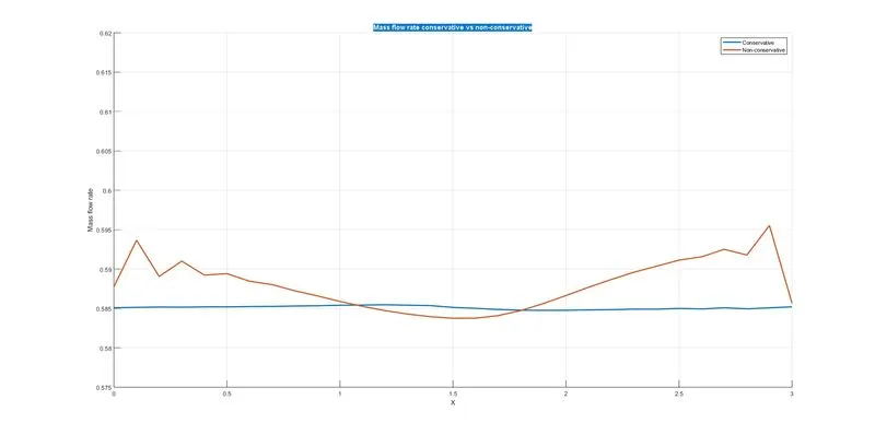
- Conservative vs Non-conservative
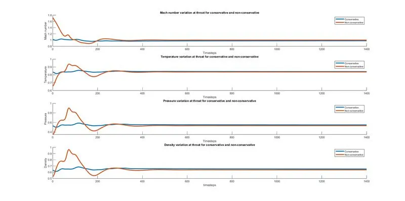
- Flow parameters non-conservative plotes
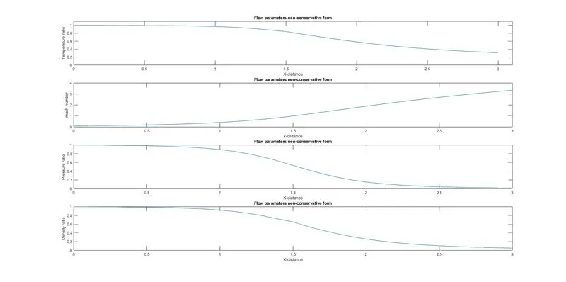
- Flow parameters non-conservative form
- Mass flow rate vs Time-step non-conservative form
- Conservative flow parameters
- Temperature vs time-step conservative form
Conclusion:
- In conclusion, the simulation of isentropic flow through a quasi 1D nozzle using MacCormack's technique revealed steady-state temperature distribution and compared conservative and non-conservative forms, providing valuable insights into compressible flow behavior.
- The grid independence test showed that both forms yield similar results with increasing resolution. Time-wise variations revealed the convergence to steady-state solutions. The comparison of mass flow rate distributions highlighted the differences between the two forms and their impact on nozzle performance. Overall, the MacCormack's technique provided a robust and accurate method for simulating supersonic nozzle flows.