Week 5 - Genetic Algorithm
Aim: To optimize the stalagmite function and find the global maxima of the function using MATLAB.
Objective:
- To optimize the stalagmite function and find the global maxima of a function.
- The concept of genetic algorithm and the Syntax for genetic algorithm.
- The plotting of studies for F maximum vs number of iterations.
Theory:
- Genetic Algorithm:- The genetic algorithm is a method for solving both constrained and unconstrained optimization problems that is based on natural selection, the process that drives biological evolution. The genetic algorithm repeatedly modifies a population of individual solutions.
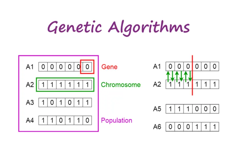
- Notion of Natural Selection:- The process of natural selection starts with the selection of fittest individuals from a population. They produce offspring which inherit the characteristics of the parents and will be added to the next generation. If parents have better fitness, their offspring will be better than parents and have a better chance at surviving. This notion can be applied to a search problem. We consider a set of solutions for a problem and select the set of best ones out of them.
Five phases are considered in genetic algorithm:-
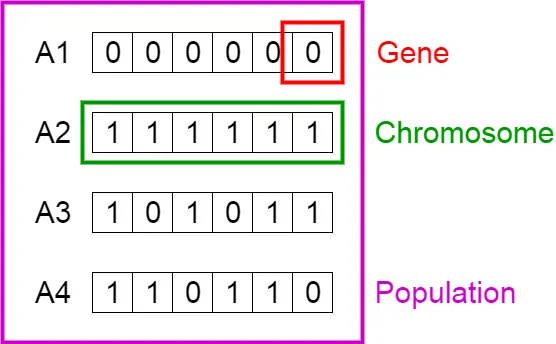
1. Initial Population:- The process begins with a set of indivisible which is called as Population. Each individual is a solution to the problem you want to solve. An indivisible gene is characterized by a set of parameters known as genes. Genes are joint into a string to form a Chromosome.
-
Population, Chromosomes and Genes
2. Fitness Function:- The fitness function determines how fit an individual is (the ability of an individual to complete with other individuals). It gives a fitness score to each individual. The probability that an individual will be selected for reproduction is based on its fitness score.
3. Selection:- The idea of selection phase is to select the fittest individuals and let them pass their genes to the next generation. Two pairs of individuals(parantes) are selected based on their fitness scores. Individuals with high fitness have more chances to be selected for reproduction.
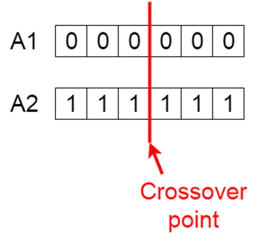
4. Crossover:- Crossover is the most significant phase in a genetic algorithm. For each pair of parents to be mated, a crossover point is chosen at random from within the genes.
-
Crossover point
5.Offspring:- Offspring are created by exchanging the genes of parents among themselves until the crossover point is reached.
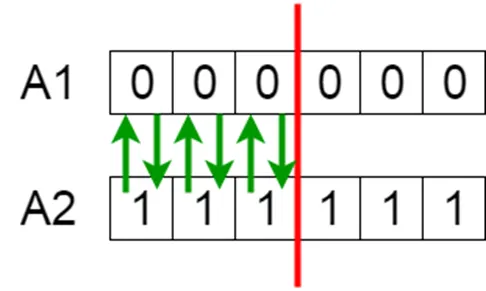
- Exchanging genes among parents
6.The new offspring are added to the population.
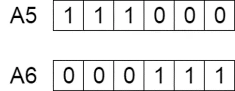
- New offspring
7.Mutation:- In certain new offspring formed, some of their genes can be subjected to a mutation with a low random probability. This implies that some of the bits in the bit string can be flipped.
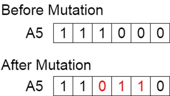
- Mutation: Before and After.
- Mutation occurs to maintain diversity within the population and present premature convergence.
Syntax for Genetic Algorithm:-
- x= ga(fun,nvars,A,b)finds a local minimum x to fun, subject to the linear inequalities A*x ≤ b. ga evaluates the matrix product A*x as if x is transposed (A*x').
- x= ga(fun,nvars,A,b,Aeq,beq) finds a local minimum x to fun, subject to the linear equalities Aeq*x = beq and A*x ≤ b. (Set A=[] and b=[] if no linear inequalities exist.) ga evaluates the matrix product Aeq*x as if x is transposed (Aeq*x').
- x= ga(fun,nvars,A,b,Aeq,beq,lb,ub) defines a set of lower and upper bounds on the design variables, x, so that a solution is found in the range lb ≤ x ≤ ub. (Set Aeq=[] and beq=[] if no linear equalities exist.)
- x= ga(fun,nvars,A,b,Aeq,beq,lb,ub,nonlcon) subjects the minimization to the constraints defined in nonlcon. The function nonlcon accepts x and returns vectors C and Ceq, representing the nonlinear inequalities and equalities respectively. ga minimizes the fun such that C(x) ≤ 0 and Ceq(x) = 0. (Set lb=[] and ub=[] if no bounds exist.)
- x= ga(fun,nvars,A,b,Aeq,beq,lb,ub,nonlcon,options) minimizes with the default optimization parameters replaced by values in options. (Set nonlcon=[] if no nonlinear constraints exist.) Create options using optimoptions.
- x= ga(fun,nvars,A,b,Aeq,beq,lb,ub,nonlcon,intcon) or x = ga(fun,nvars,A,b,Aeq,beq,lb,ub,nonlcon,intcon,options) requires that the variables listed in intcon take integer values.
- x= ga(problem) finds the minimum for problem, a structure described in problem.
- [x,fval] = ga(___), for any previous input arguments, also returns fval, the value of the fitness function at x.
- [x,fval,exitflag,output] = ga(___)also returns exitflag, an integer identifying the reason the algorithm terminated, and output, a structure that contains output from each generation and other information about the performance of the algorithm.
- [x,fval,exitflag,output,population,scores] = ga(___)also returns a matrix population, whose rows are the final population, and a vector scores, the scores of the final population.
Governing Equations
Stalagmite Function
where, `f(x,y) = f1,xf2,xf1,yf2,y`
`therefore``f1,x=[sin(5.1pix+0.5)]^6`
`f1,y=[sin(5.1piy+0.5)]^6`
`f2,x=exp[-4ln(2)(x-0.0667)^2/0.64]`
`f2,y=exp[-4ln(2)(y-0.0667)^2/0.64]`
Matlab Code:
- Stalagmite Function code
function f = stalagmite_fun(input_vector) x = input_vector(1); y = input_vector(2); f1 = (sin(5.1*pi*x+0.5))^6; f2 = (sin(5.1*pi*y+0.5))^6; f3 = exp(-4*log(2)*((x-0.0667)^2)/0.64); f4 = exp(-4*log(2)*((y-0.0667)^2)/0.64); f = -(f1*f2*f3*f4); end - Genetic Algorithm Code with all three cases.
clear all
close all
clc

% Defining our search space
x = linspace(0, 0.6, 150);
y = linspace(0, 0.6, 150);

% Creating a 2Diamenshional mesh
[xx,yy] = meshgrid(x,y);

% Evaluating the stalagmite
for i = 1:length(xx)
    for i= 1:length(yy)
        input_vector(1) = xx(i,i);
        input_vector(2) = yy(i,i);
        f(i,i) = stalagmite_fun(input_vector);
    end
end

% Study 1 Unbounded Inputs
num_case = 150;

 for i = 1:num_case
    [inputs, fopt(i)] = ga(@stalagmite_fun,2);
    xopt(i) = inputs(1);
    yopt(i) = inputs(2);
end

figure(1)
subplot(2, 1, 1)
hold on
surfc(x,y,-f)
shading interp
plot3(xopt, yopt, -fopt, 'Marker','o', 'MarkerSize',5, 'MarkerFaceColor','r')
title('Unbounded Inputs')
subplot(2, 1, 2)
plot(-fopt)
xlabel('Iterations')
ylabel('Function Minimum')


% Study2 Bound Inputs

tic
for i = 1:num_case
    [inputs, fopt(i)] = ga(@stalagmite_fun,2,[],[],[],[],[0;0],[0.6;0.6]);
    xopt(i) = inputs(1);
    yopt(i) = inputs(2);
end
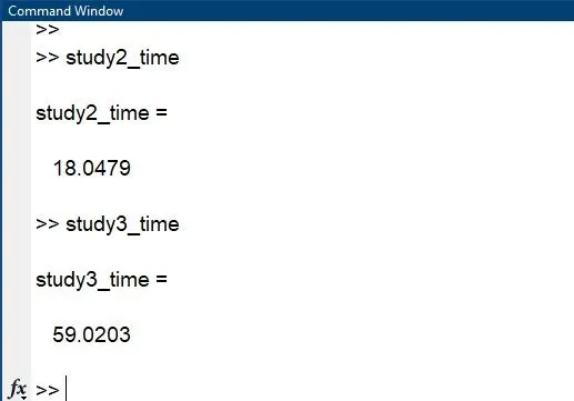
study2_time = toc;

%Plotting
figure(2)
subplot(2,1,1)
hold on
surf(x,y,-f)
shading interp
plot3(xopt,yopt,-fopt,'marker','o','MarkerSize',5,'MarkerFaceColor','r')
title('Bounded Case')
subplot(2,1,2)
plot(-fopt)
xlabel('No. Of Iteration')
ylabel('Function Maximum Value')

% Study3 Increase Population

options = optimoptions('ga');
options = optimoptions(options,'PopulationSize',300);

tic
for i = 1:num_case
    [inputs,fopt(i)] = ga(@stalagmite_fun,2,[],[],[],[],[0;0],[0.6;0.6],[],[],options);
    xopt(i)= inputs(1);
    yopt(i) = inputs(2);
end
study3_time = toc;

figure(3)
subplot(2,1,1)
hold on
surf(x,y,-f)
shading interp
plot3(xopt,yopt,-fopt,'marker','o','MarkerSize',5,'MarkerFaceColor','r')
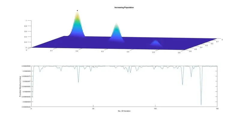
title('Increasing Population')
subplot(2,1,2)
plot(-fopt)
xlabel('No. Of Iteration')
ylabel('Function Maximum Value')
Explanation of code:
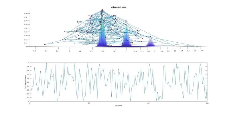
- Study 1:- The unbounded input is provided for calculating the value of global maxima.
- We had to provide the input value for ga syntax and global maxima for unbounded case and use the stalagmite function to find the unbounded case using the num case command.
-
% Defining our search spacex = linspace(0, 0.6, 150);y = linspace(0, 0.6, 150);% Creating a 2Diamenshional mesh[xx,yy] = meshgrid(x,y);% Evaluating the stalagmitefor i = 1:length(xx)for i= 1:length(yy)input_vector(1) = xx(i,i);input_vector(2) = yy(i,i);f(i,i) = stalagmite_fun(input_vector);endend% Study 1 Unbounded Inputsnum_case = 150;for i = 1:num_case[inputs, fopt(i)] = ga(@stalagmite_fun,2);xopt(i) = inputs(1);yopt(i) = inputs(2);endfigure(1)subplot(2, 1, 1)hold onsurfc(x,y,-f)shading interpplot3(xopt, yopt, -fopt, 'Marker','o', 'MarkerSize',5, 'MarkerFaceColor','r')title('Unbounded Inputs')subplot(2, 1, 2)plot(-fopt)xlabel('Iterations')ylabel('Function Minimum')
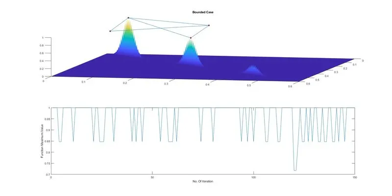
- Study 2:- The bounded inputs provide for calculating the value of global maxima.
- For boundedinputs we had the value for num case. For the bounded case we use 'for loop' for repeated values. The surf command was also used to plot the graph in three dimensions.
-
ticfor i = 1:num_case[inputs, fopt(i)] = ga(@stalagmite_fun,2,[],[],[],[],[0;0],[0.6;0.6]);xopt(i) = inputs(1);yopt(i) = inputs(2);endstudy2_time = toc;%Plottingfigure(2)subplot(2,1,1)hold onsurf(x,y,-f)shading interpplot3(xopt,yopt,-fopt,'marker','o','MarkerSize',5,'MarkerFaceColor','r')title('Bounded Case')subplot(2,1,2)plot(-fopt)xlabel('No. Of Iteration')ylabel('Function Maximum Value')
- Study 3:- The bounded inputs provided the many values of population size for better optimization in order to calculate the value of global maxima.
- We used the bounded input to find the global maxima using the options population and used ga syntax of the stalagmite function. The 'shading interp' is used to remove the grid line which was on the mountains on the graph. The time taken was also calculated using the 'tic-toc' command.
-
options = optimoptions('ga');options = optimoptions(options,'PopulationSize',300);ticfor i = 1:num_case[inputs,fopt(i)] = ga(@stalagmite_fun,2,[],[],[],[],[0;0],[0.6;0.6],[],[],options);xopt(i)= inputs(1);yopt(i) = inputs(2);endstudy3_time = toc;figure(3)subplot(2,1,1)hold onsurf(x,y,-f)shading interpplot3(xopt,yopt,-fopt,'marker','o','MarkerSize',5,'MarkerFaceColor','r')title('Increasing Population')subplot(2,1,2)plot(-fopt)xlabel('No. Of Iteration')ylabel('Function Maximum Value')
Result:
For Unbounded input
For Bounded Inputs
For Bounded Inputs With Population Size
- Study time for cases are
- Study time for case 2 is 18.0479
- Study time for case 3 is 59.0203
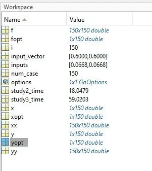
- The Global maxima of the function is 0.0668
CONCLUSION:
- By using ga syntax we got the stalagmite plot. And optimize the population.
- The global maxima. Is calculated by population of the solution from the obtained value
Reference:-