Week 4.1 - Solving second order ODEs

Aim: To solve a second-order difference equation.

Objective:

• To write a program that solves the following ODE.
• This ODE represents the equation of motion of a simple pendulum with damping.

Theory:

• Ordinary Differential Equations (ODEs) - The term ordinary is used in contrast with the term partial differential equation which may be with respect to more than one independent variable An Ordinary differential equation (ODE) is a differential equation containing one or more functions of one independent variable and the derivatives of those functions. .
• Simple pendulum consists of a bob of a mass. `m` attached to a cord of length `l` that can freely oscillate in the gravitational field. The simple pendulum is a simplified model of a number of real-life systems.

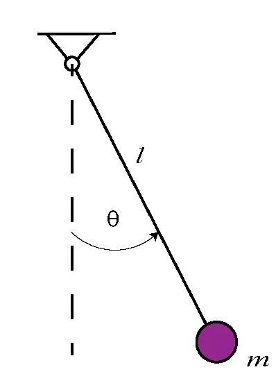
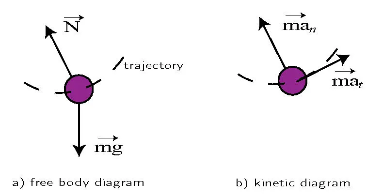
The equation of motion of a simple pendulum with damping is

`(d^2theta)/dt^2+b/m*(d theta)/dt+g/l*sin theta=0`

In above equaction

`g`= gravity in m/s2,

`l` = length of the pendulum in m,

`m` = mass of the ball in kg ,

`b` = damping coefficient.

Inputs

`g` = 9.81m/s2

`l` = 1 meter

`m` = 1kg

`b` = 0.05

For angular displacement=0,

Angular velocity=3 rad/sec at time t=0.

CODE

1) ODEs function code:

function [dtheta_dt] = ode_func(t, theta, b, g, L, m)
    
        theta1 = theta(1)
        theta2 = theta(2)
        dtheta1_dt = theta(2)
        dtheta2_dt = -(b/m)*theta2 - (g/L)*sin(theta1)
        dtheta_dt = [dtheta1_dt; dtheta2_dt]
end

2) ODEs main code:

clear all
close all
clc

% Inputs
    b = 0.05;
    g = 9.81;
    L = 1;
    m = 0.1;

 % Initial Condition 
        theta_0 = [0;5];

 % Time Point    
        t_span = linspace(0,10,500);

% Solve ode 
        [t, results] = ode45(@(t,theta) ode_func(t, theta, b, g, L, m),t_span, theta_0);
% Plot 
    plot(t,results(:,1));
    hold on;
    plot(t,results(:,2));
    xlabel('Time');
    ylabel('Plot');
    grid on

% Plotting the movie
  ct = 1; 
    for i = 1:length(results(:,2)) 
        x = 0; 
        y = 0; 
        x1 = L*sin(results(i,1)+pi); 
        y1 = L*cos(results(i,1)+pi); 

    figure(2) 
        plot([x x1],[y y1],'-o','MarkerSize',15,'MarkerFaceColor','r','MarkerEdgeColor','b','linewidth',3)
        axis([-1.1 1.1 -1.2 0.4]) 
        hold on 
        plot([-1 1],[0 0],'linewidth',5) 
        M(ct) = getframe(gcf);
        hold off 
         ct = ct + 1; 
end
    
    movie(M)
    videofile = VideoWriter('Pendulum animation','Uncompressed AVI');
    open(videofile)
    writeVideo(videofile,M)
    close(videofile)

Code explanation

• Clear all, close all, clc :- this command is used to clear all the code which is running and close all is used to close all opened running programs.
• t_span:- this command is a solver which specifies the time span of the loop that is going to solve the ordinary differential equation.
• ODEs:- is a function that solves a differential equation using a numerical method, the highest order is 2. The function takes at least 2 inputs to solve the equation to result. The ODEs is a syntax of a ‘ode45’ solver.

• Mark:- is used to create a sphere.
• Hold on:- is used to hold all reading in one frame.
• Movie (M):- is used to create a film of motion of a pendulum.
• VideoWriter:- command specifies the name of the file and type of file data .
• Open:- is used to open the file.
• Close:- is used to close the video file.

Splitting of Second order differential equation

`therefore``(d theta)/(dt) = (d theta1)/dt = theta2`

`therefore``(d^2 theta)/dt = (d^2 theta1)/dt^2 = d/dt ((d theta1)/dt ) = d/dt (theta2)`

`therefore` `(d^2 theta )/dt^2 +b/m* (d theta1)/dt +g/l sin theta 1 = 0`

`therefore` `(d theta 2)/dt + b/m *(d theta1 )/dt +g/l *sin theta = 0`

`therefore``(d theta 2 )/dt = - B/m theta 2 - g/l sin theta 1`

Error faced while programming:-

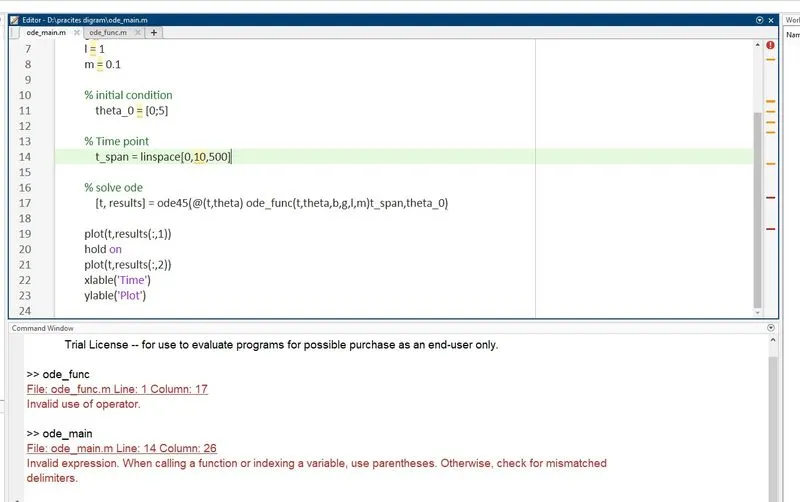
• Invalid expression

.

solution :-

1. I had used square brackets instead of round brackets in the linspace command.
2. The code of function was not saved before I run the program, and I had miss spell the spelling of function.

Result

• The output plot has been obtained for plot vs time.

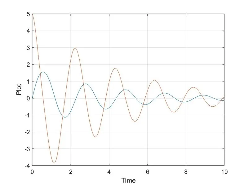
The link for Animation of simple pendulum:-

https://youtu.be/yz2XizjmCDk

Conclusion:-

• The second order is reduced to a simple differential equation where it is easy to solve the given equation.
• The animation is created by using an ode45 solver at different points of the motion of the simple pendulum.